I spent the first semester in Berkeley Formula Electric Autonomous working on a RRT* based approach to solving the path planning problem. I soon discovered the is a much faster, more efficient, more accurate, and more customizable way through optimization. This is my explanation of how optimization works, and how it is used in the team.
There are 3 main parts of the autonomous pipeline:
- Perception
- SLAM
- Path planning
- Model Predictive Control (MPC)
Optimization can be used to solve SLAM (graph SLAM), path planning, and MPC.
I will be mostly talking about the path planning solution.
Here are explanations for the math behind convex optimization. EECS127 course reader This Tutorial
Here is Reid’s explanation.
The essence of this approach is phrasing the path planning problem in a specific standard way so that we can use a solver to solve the problem.
There are several libraries in python that specialize in solving optimization problems in standard form. So if we can get the problem into such a form, we can plug it into a solver and get an answer.
Lets look at one of the forms:
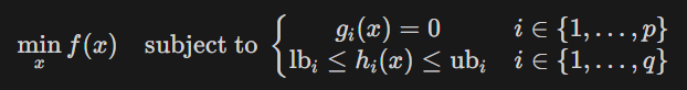
We chose either minimize or maximize (lets say minimize), and chose the quantity we want to minimize (lets say f(x)=x^2 in this case).
Then we specify any constraints we want on the variables such as x>=0 and x<=9.
We have now an optimization problem!
Now we can input it into a solver like cvxpy(what I got started with and only does convex optimization) or casadi(what the team uses and can solve non linear programs) to solve the problem.
In our example, our solution would be 0 because the smallest x^2 such that 0<= x <= 9 is 0.