For Fall 2024, I am taking an image processing class where one of the assignments involves creating panoramas by implementing image transformations. The process involves manually labeling correspondences between images and performing image warping, rectification, and blending. Below, I document my approach to this assignment with in-depth explanations of each step.
Table of Contents #
Part A: Stitching a Panorama #
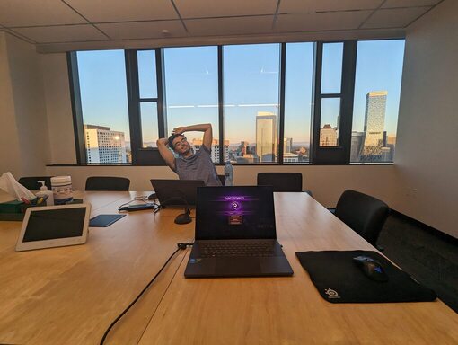
Shoot the Pictures #
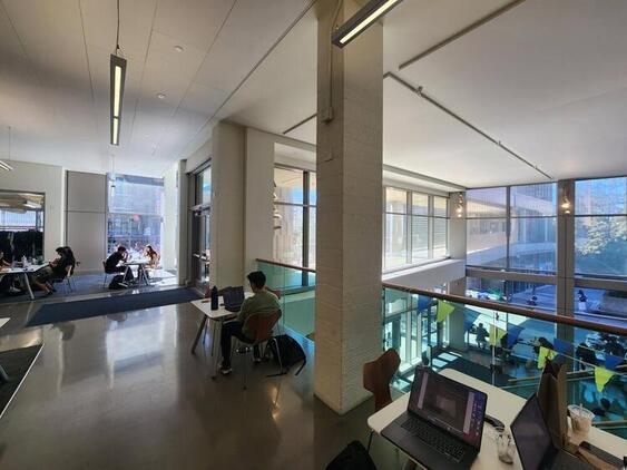
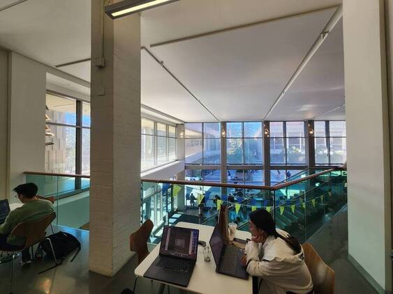
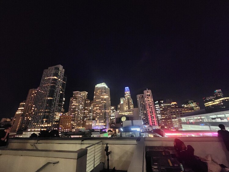
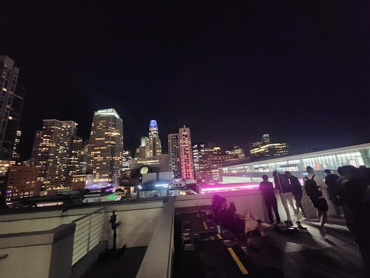
I used a Samsung Galaxy S22 with a 0.5x zoom to capture wide-angle shots. The goal is to capture overlapping images that can be aligned using homographies. Below are some of the pictures I took, which will be used for different stages of the project:
-
MLK Building
-
Night Skyline
-
Table Top
Guidelines for Capturing Images: #
- Camera Movement: Keep the center of projection fixed and rotate the camera for consistent perspective changes.
- Overlap: Ensure about 40%-70% overlap between consecutive images to make alignment easier.
- Avoid Barrel Distortion: Use lenses that avoid distortion, keeping straight lines straight.
- Lighting: Capture images in quick succession to maintain consistent lighting and reduce potential artifacts.
Recover Homographies #
Homographies are key to transforming points from one image into another. The homography matrix ( H ) is a 3x3 matrix that defines this transformation. It maps points from image 1 to image 2 based on their coordinates.
Given corresponding points ( p = (x, y) ) in the first image and ( p’ = (x’, y’) ) in the second, the transformation can be described by:
$$ p’ = H \cdot p $$
Steps to Recover Homography: #
- Select Corresponding Points: Using a manual labeling tool, I selected pairs of corresponding points in both images.
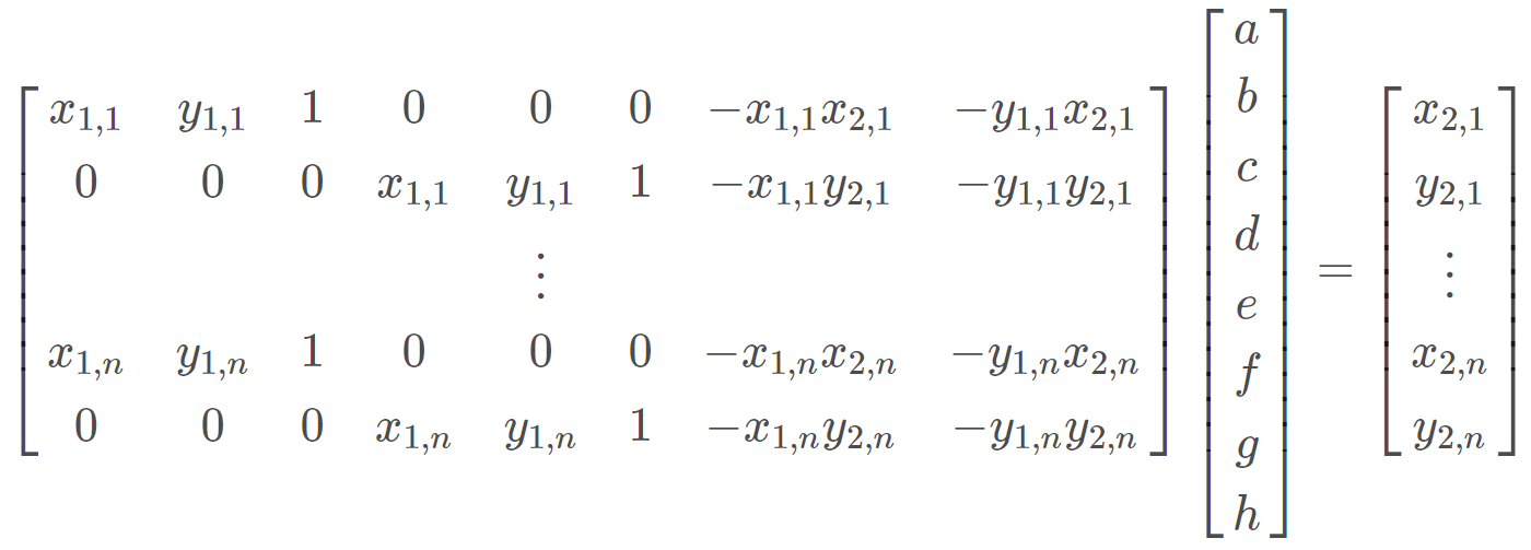
- Formulate the Equation: With four or more correspondences, the homography matrix ( H ) can be computed by solving the system ( Ah = b ), where ( A ) is a matrix formed from the correspondence pairs and ( h ) is the vectorized form of the homography matrix.
- Solve Using Least Squares: For robustness, I use more than four points, resulting in an overdetermined system. The least squares method minimizes error in finding the best-fit homography.
Since our H matrix contains 8 unknown variables (the lower-right corner of the matrix is a scaling factor and set to 1), we need >= 8 equations to solve for the matrix. Each point correspondence gives us 2 equations. So, we need at least 4 points to solve the system of linear equations. In practice, we often use lots of points to avoid an unstable and noisy transformation. Least-squares can then be used to recover the homography matrix:
Warp the Images #
Once the homography matrix ( H ) is computed, I use it to warp one image into the coordinate system of another. The warping operation applies a projective transformation, ensuring that the perspective between the images is corrected.
The warping process is defined as:
$$ p = H^{-1} \cdot p' $$
Where ( H^{-1} ) is the inverse of the homography matrix, used for inverse warping.
Key steps in warping:
- Forward vs. Inverse Warping: I used inverse warping to avoid holes in the final image, computing pixel values in the destination image by interpolating pixel values from the source.
- Interpolation: Using
cv2.remap, I performed interpolation to fill in missing pixel values smoothly.
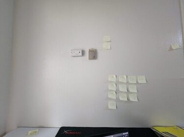
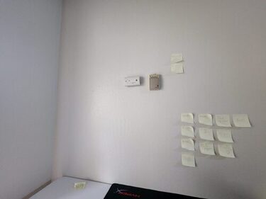
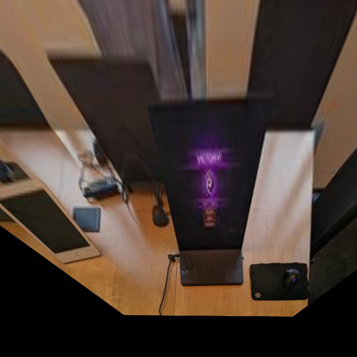
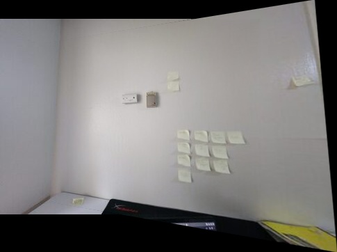
Image Rectification #
Before blending the images into a mosaic, I rectified images to ensure the correctness of the homography transformation. Rectification involves mapping an image containing a known planar surface (like a poster or keyboard) so that the plane appears front-facing.
For example:
-
Starcraft Laptop
-
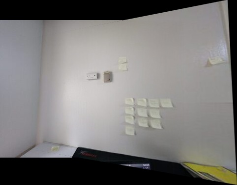
Poster


In both cases, I manually selected points on the objects and mapped them to a predefined square in the output space. This demonstrates that the warping process is functioning correctly.
Blend the Images into a Mosaic #
With the images properly aligned through homographies, the next step is to blend them into a seamless mosaic. Simple stitching often leads to harsh edges and artifacts. To avoid this, I used Weighted Distance Blending.
Weighted Distance Blending: #
After aligning the images with homographies, I needed to blend them into a seamless mosaic. Initially, I experimented with Laplacian pyramids for multi-scale blending. While this approach is effective in preserving detail and avoiding harsh transitions, it was challenging to determine the exact boundaries between overlapping images, leading to imperfect blending results.
To address this, I switched to a more straightforward and effective method: weighted feathering using the bwdist function. This method worked exceptionally well and produced smooth transitions between the overlapping regions of the images.
Weighted Feathering with bwdist
#
The idea behind this technique is to compute a distance transform for each image, which measures the distance from the nearest edge of the mask. The further a pixel is from the boundary, the more weight it carries in the blending process. The weights are normalized to smoothly transition between the two images based on their distances from the edges.
Here’s the Python code I used for blending:
def bwdistBlend(panorama, enlarged_image):
    # Create binary masks for each image
    mask_2 = np.any(enlarged_image > 0, axis=-1).astype(np.float32)
    mask_1 = np.any(panorama > 0, axis=-1).astype(np.float32)

    # Compute the intersection mask where both images overlap
    intersection = np.logical_and(mask_1, mask_2)
    # Compute distance transform for both masks (distance from zero)
    dist_1 = bwdist(mask_1)
    dist_2 = bwdist(mask_2)

    # Normalize distance maps to range [0, 1]
    dist_1_norm = dist_1 / (dist_1.max() + 1e-8)
    dist_2_norm = dist_2 / (dist_2.max() + 1e-8)

    # Compute the blend weights based on distance transforms
    blend_weights_1 = dist_1_norm / (dist_1_norm + dist_2_norm + 1e-8)
    blend_weights_2 = dist_2_norm / (dist_1_norm + dist_2_norm + 1e-8)

    # Ensure the blend weights are only applied in the overlapping regions
    blend_weights_1[~intersection] = 1  # Only panorama where no intersection
    blend_weights_2[~intersection] = 0  # Only enlarged_image where no intersection

    # Blend the two images using the computed weights
    result = panorama + enlarged_image
    result[intersection] = (panorama.astype(np.float32) * blend_weights_1[:, :, np.newaxis] +
              enlarged_image.astype(np.float32) * blend_weights_2[:, :, np.newaxis])[intersection]

    # Clip the result to ensure valid pixel values and convert back to uint8
    result = np.clip(result, 0, 255).astype(np.uint8)

    return result
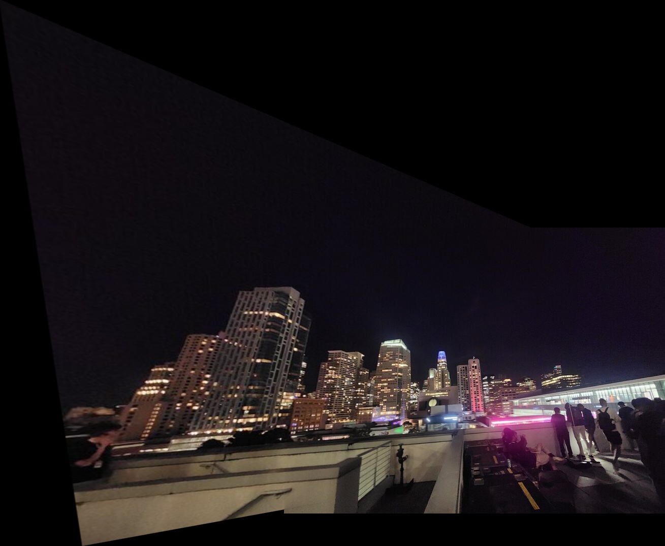
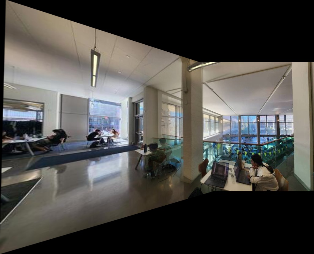
Here are the final mosaics:
-
Night Skyline Mosaic
-
MLK Building Mosaic
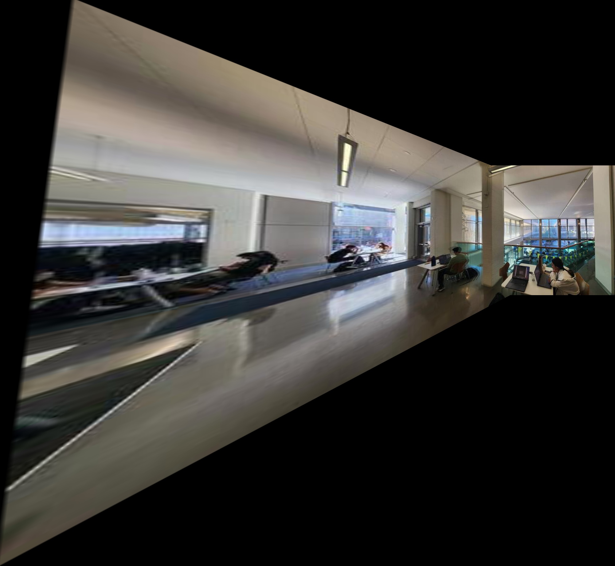
-
Table Mosaic
Part B: Automatic Feature Detection and Matching #
In this part, we implement automatic feature detection and matching to create panoramas without manual correspondence selection. We’ll follow the approach outlined in “Multi-Image Matching using Multi-Scale Oriented Patches” by Brown et al., with some simplifications.
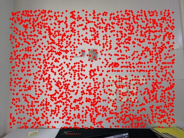
1. Harris Corner Detection #
The first step is detecting corner features using the Harris corner detector. These are regions with high contrast that exhibit significant changes in both horizontal and vertical directions.
Implementation Details:
- Used single-scale Harris corner detection
- Threshold set to maintain strong corner responses
Results:
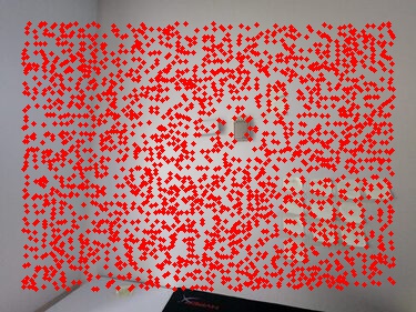
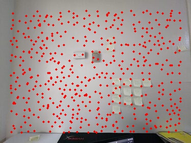
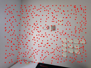
2. Adaptive Non-Maximal Suppression (ANMS) #
To ensure a good spatial distribution of features and filter out weaker corners, I implemented ANMS as described in Section 3 of the paper.
Implementation Details:
- Computed suppression radius for each point
- Sorted points by the maximum radius that the point is the most “cornery” determined by harris corner detection value. Then picked to the top few points.
- This maintains even spatial distribution while preserving strongest features
Results:
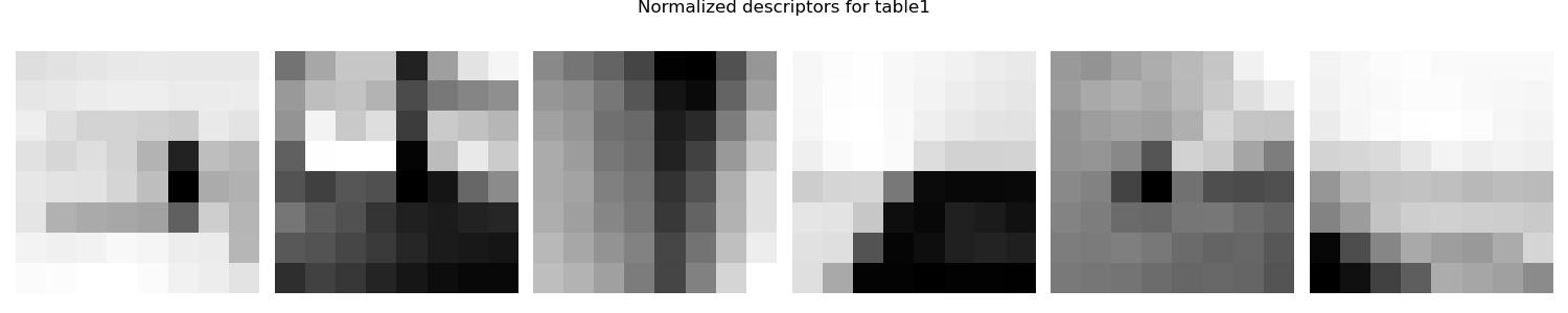
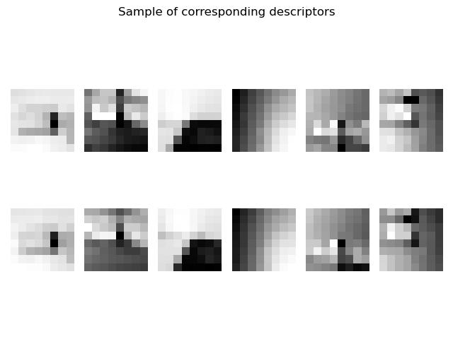
3. Feature Descriptor Extraction #
For each detected corner, I created a distinctive feature descriptor to enable matching. (idea is that we want the first nearest neighbor to be super close and the second nearest neighbor to be super far)
Implementation Details:
- Extracted 40x40 patches around each corner
- Downsampled to 8x8 descriptors to handle noise
- Applied bias/gain normalization
- Used axis-aligned patches (no rotation invariance)
Example Normalized Descriptors:
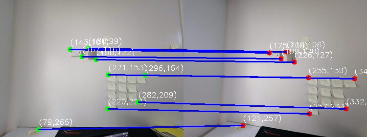
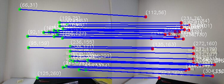
4. Feature Matching #
Implemented feature matching using Lowe’s ratio test between first and second nearest neighbors.
Implementation Details:
- Computed distances between all descriptor pairs
- Applied ratio test for matching uniqueness
- Used threshold based on Figure 6b from the paper
Matched Descriptor Examples:
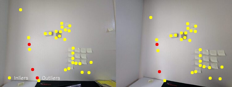
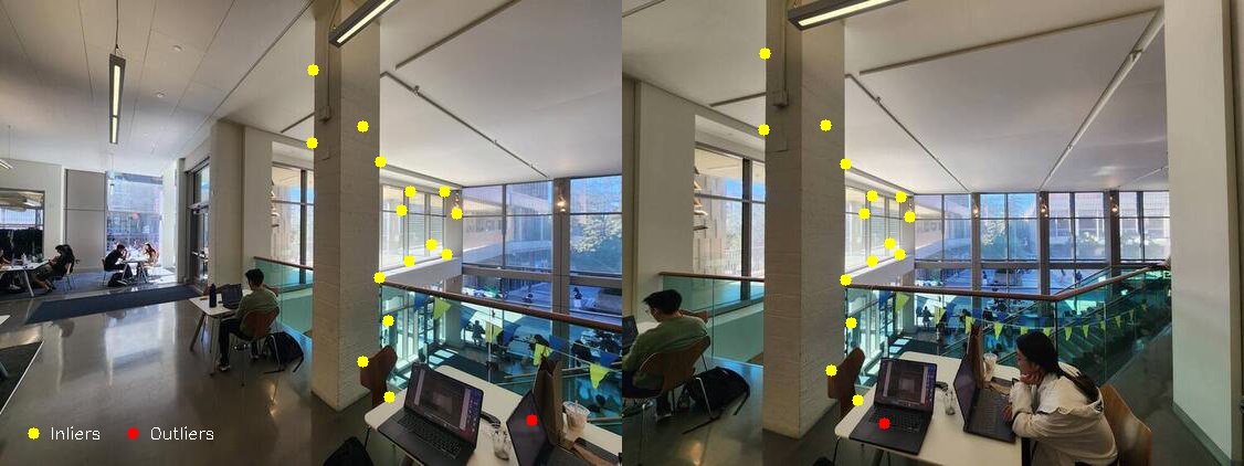
5. RANSAC Homography Estimation #
Used RANSAC to robustly estimate the homography transformation between images.
Implementation Details:
- Randomly sampled 4 point correspondences
- Computed homography for each sample
- Counted inliers using distance threshold
- Refined homography using all inliers
RANSAC Results:
- Yellow points: Inliers
- Red points: Outliers
Manual vs. Automatic Comparison #
Here’s a side-by-side comparison of the results from manual and automatic stitching for all three scenes:
MLK Building #
Manual:
Night Skyline #
Manual:
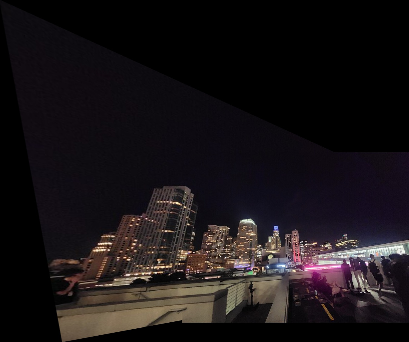
Table Scene #
Manual:
Analysis of Results: #
- Accuracy: Both methods produced well-aligned panoramas, with the automatic method showing comparable accuracy to manual selection. Both methods struggle with the MLK panorama as the overlap region is small and the transformation is large.
- Efficiency: Automatic method is extremely fast
- Edge Cases: Manual method can sometimes handle cases where automatic detection fails (the manual one in the mlk example looks better)
Correspondence Comparison: Manual vs. Automatic #
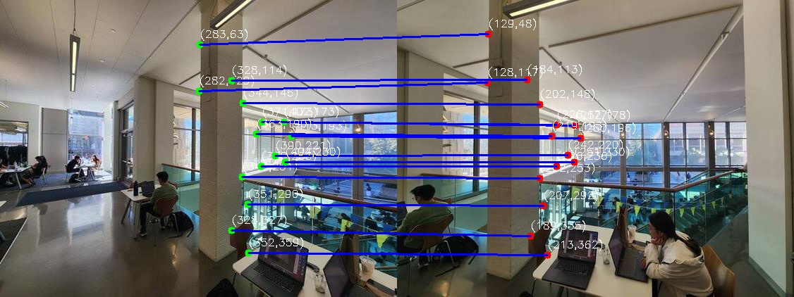
MLK Building #
Manual Correspondences:
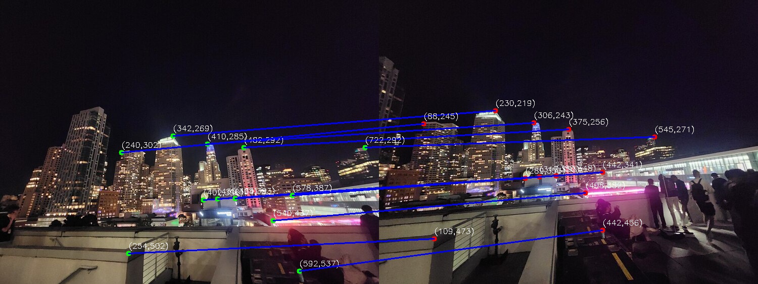
Night Skyline #
Manual Correspondences:
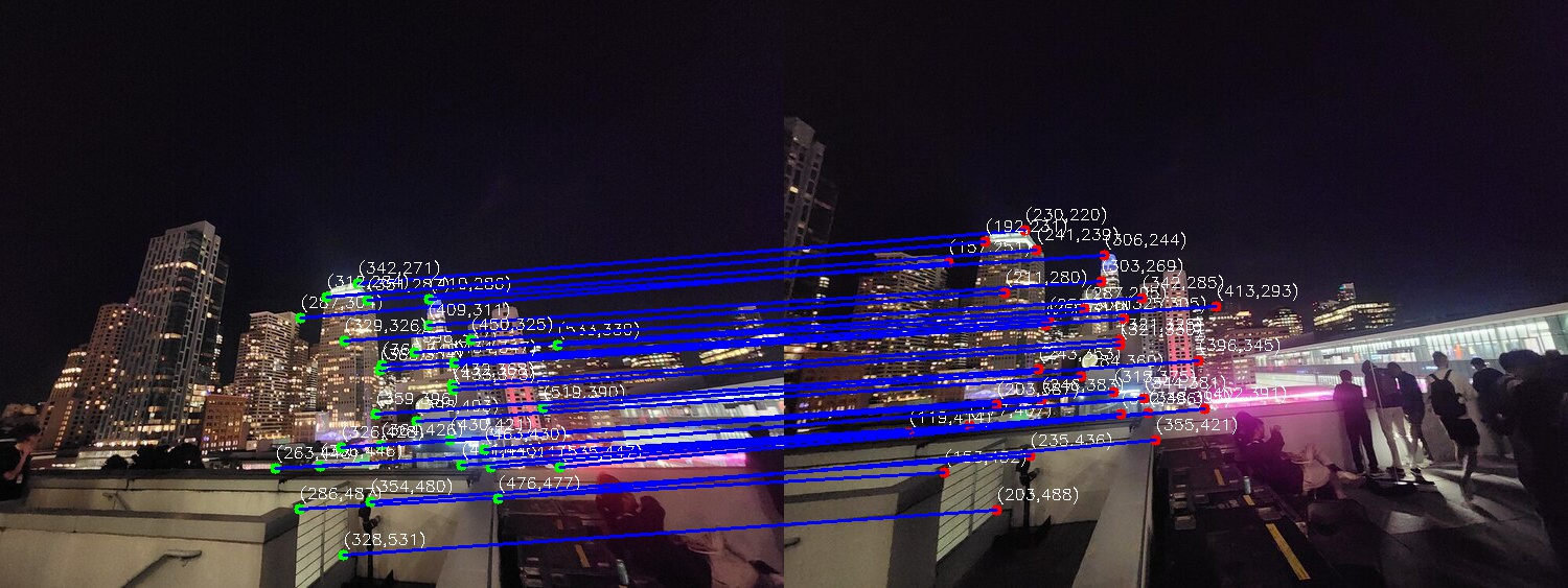
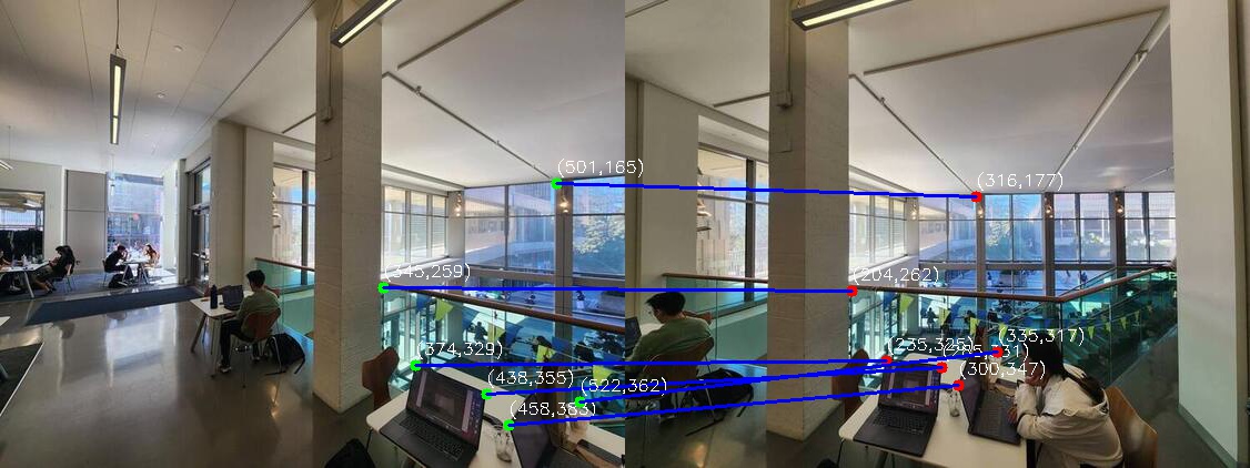
Table Scene #
Manual Correspondences:
Analysis of Correspondence Methods: #
Manual Correspondence Selection #
Advantages:
- High precision in selecting specific features
- Ability to choose semantically meaningful points (e.g., corners of windows, distinctive architectural features)
- Works well in low-texture or repetitive regions where automatic methods might struggle
- Can handle cases with significant lighting changes
Disadvantages:
- Time-consuming process
- Subject to human error
- Limited number of correspondences (typically 8-12 points)
Automatic Correspondence Detection #
Advantages:
- Much faster execution
- Generates many more correspondences
- Consistent results across multiple runs
- Evenly distributed points across the image due to ANMS
Disadvantages:
- Can be fooled by repetitive patterns
- Sensitive to parameter tuning (Harris threshold, ANMS radius, matching ratio)
- May produce some incorrect matches (though RANSAC helps filter these)
- Requires sufficient texture in the images
Impact on Final Results: #
- Alignment Quality: Both methods produced well-aligned panoramas.
- Processing Time: Manual method took about 2-3 minutes per image pair for point selection, while automatic method runs in seconds
- Reliability: The manual selection was more reliable for challenging cases
- Point Distribution: Automatic method achieved better spatial distribution of points thanks to ANMS, while manual selection often concentrated on obvious features
What I Learned #
The coolest thing I learned from this project was how robust feature matching can be achieved through RANSAC. It’s fascinating that Lowe’s ratio test and RANSAC can get correspondances that rival human labling. The process of seeing random corner points transform into meaningful correspondences through these algorithmic steps was particularly enlightening.
Code #
You can find the full implementation of my project here.