Path Planning with NLP

Path planning is the challenge of calculating the best path for a race car to take through a given track.

Here is the goal (video from another team):

Notice how the car planned the optimal path around that track the instant it completed the first lap.

The example output below from my implementation solves for the positions, velocity, and orientation of the car at every point in the optimal path (racing line).

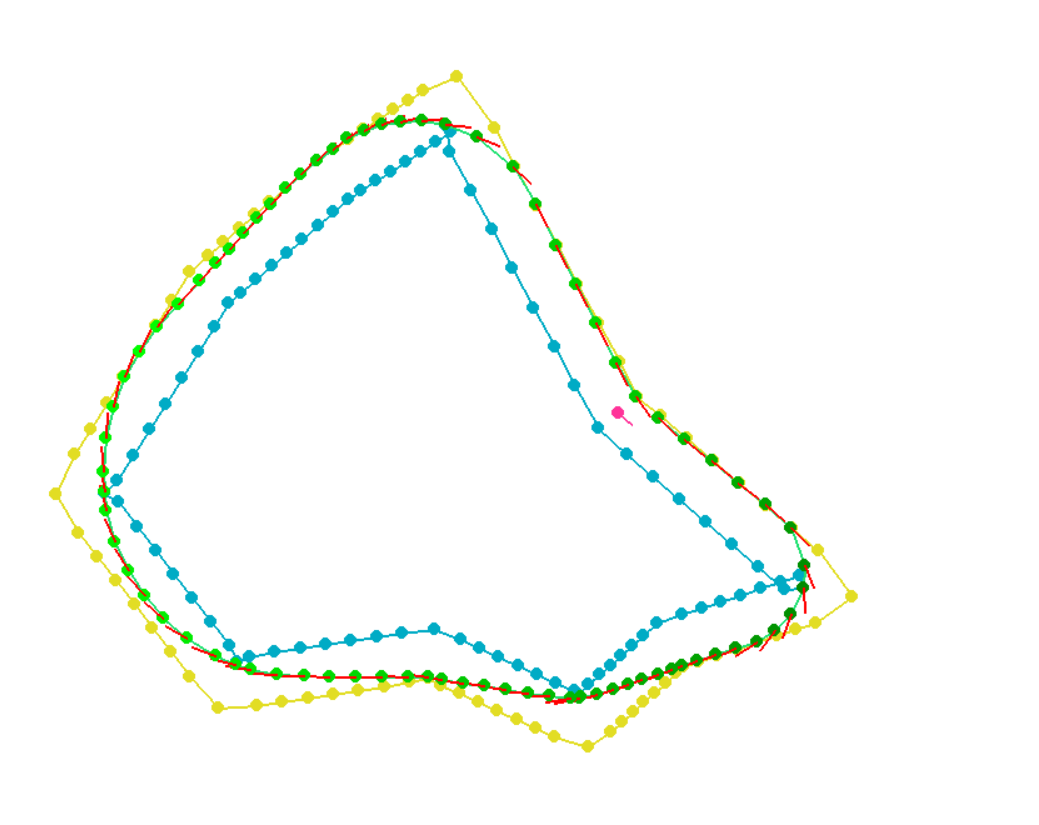
Notice the light/dark color of green signifying faster, slower regions, as well as the red lines indicating the heading of the car.

After developing an RRT* based approch to path planning, my friend Reid Dye introduced me to a Non-Linear programming based way to solve the problem. It was faster, more accurate, more custamizable with things like friction and velocity constraints, and overall more organized.

Here is a summary.

Final solution Link to heading

There are a bunch of paths beyond the first track example that folded in on itself but that is because the initial guess pointed the car looking backwards and so it did not converge to the right local minimum. This could be fixed with a better initial guess (start off looking towards the midpoint of the next section) to guerentee convergence.

After solving for the path with a few points, a subdivide algorithm breakes the path into 0.1 second increments so we have many datapoints in the final path.

If there is a steep angle in the track, the initial guess of the heading may be looking the opposite way as it should be, and this usually confuses the solver to converging to an infeasible solution. This is solvable with a smarter intial guess, but its not a fun problem so I decided not to resolve the issue.

How it works Link to heading

Reid has made a good explanation of the approach for the team.

My implimentation assumes constant wheel torque with fixed max velocity and max acceleration. I also assume a constant acceleration envelope.

The process Link to heading

Here are the issues I faced along the way:

• I expllicitly solved for the vehicle dynamics (with sinh and cosh), so the dynamics of the car had a division by 0 when the steering was set to 0. This led to the solver crashing when it got near steering = 0. The solution was to phrase the dynamics as an initial value problem with differential equations, then letting casadi solve for the function.

def continuous_dynamics_fixed_x_order(x, u, car_params={'l_r': 1.4987, 'l_f':1.5213, 'm': 1.}):
        """Defines dynamics of the car, i.e. equality constraints.
        parameters:
        state x = [xPos,yPos,v,theta]
        input u = [F,phi]
        """
        beta = arctan(car_params['l_r']/(car_params['l_f'] + car_params['l_r']) * tan(u[1]))
        xdot = x[2]*cos(x[3] + beta)
        ydot = x[2]*sin(x[3] + beta)
        vdot = u[0]
        thetadot = x[2] / car_params['l_r'] * sin(beta)

        return vertcat(xdot,
                        ydot,
                        vdot,  
                        thetadot)                 
    
    def discrete_custom_integrator(n = 3, car_params={'l_r': 1.4987, 'l_f':1.5213, 'm': 1.}):
        x0 = MX.sym('x0', 4)
        u = MX.sym('u', 2)
        dt = MX.sym('t')
        xdot = NLPSolver.continuous_dynamics_fixed_x_order(x0, u, car_params)
        f = Function('f', [x0, u], [xdot])
        
        x = x0
        for i in range(n):
            xm = x + f(x, u)*(dt/(2*n))
            x = x+f(xm, u)*(dt/n)
        return Function('integrator', [x0, u, dt], [x])

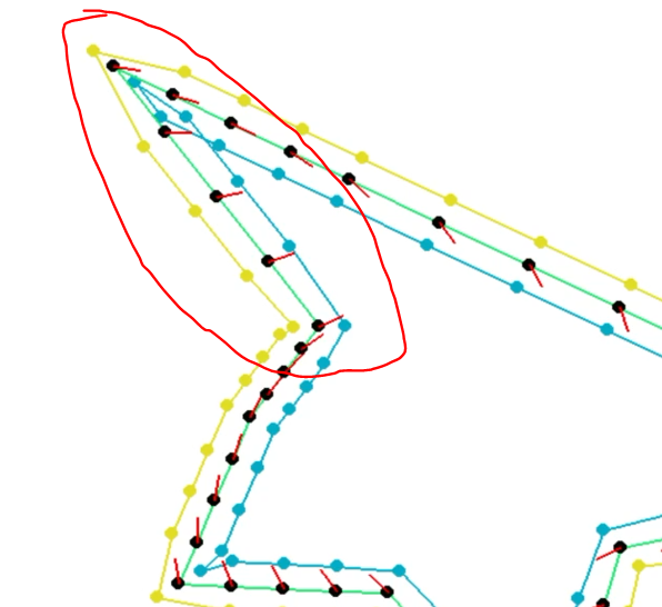
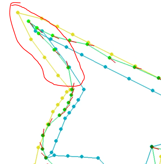
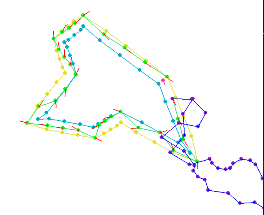
• The solver kept on converging to a local infeasable point, and the path it showed was completely ignoring the dynamics of the car. It turns out I was passing in the first control input for every single dynamics calculation regrdless of which point I was trying to calculate (I messed up u[i, :] vs u[:, i]). The purple path below is the path produced based on the dynamics of the car and control inputs (you can see it differs from the outputted path). The problem is simple, but took me way too long to catch. I even made a game so I could control a car following the dynamics using arrow keys to test my dynamics.

• The initial guess has to be a pretty good guess. The most straightforward method of making an initial guess is following the midpoints, and setting the headings to just rotate from 0 to 2pi. However, if there is a steep angle in the track, the initial guess of the heading may be looking the opposite way as it should be, and this usually confuses the solver to converging to an infeasible solution.