Everything is KL minimization: The Current Autoregressive Video Generation Landscape

The forward process gradually corrupts data $x_0 \sim q(x_0)$ by adding Gaussian noise over $T$ timesteps:

where $\beta_1, \ldots, \beta_T$ is a variance schedule controlling how much noise to add at each step.

The beauty of Gaussian noise is that we can sample $x_t$ directly from $x_0$ in closed form:

where $\alpha_t = 1 - \beta_t$ and

This means $x_t = \sqrt{\bar{\alpha}_t} x_0 + \sqrt{1 - \bar{\alpha}_t} \epsilon$ where $\epsilon \sim \mathcal{N}(0, I)$.

As $t \to T$, $\bar{\alpha}_t \to 0$ and $x_t$ approaches pure Gaussian noise.

The backward process learns to reverse the diffusion:

Starting from $x_T \sim \mathcal{N}(0, I)$, we iteratively denoise: $x_T \to x_{T-1} \to \cdots \to x_0$.

The full generative process is:

We want to maximize the log-likelihood $\log p_\theta(x_0)$, but this is intractable. Instead, we maximize the Evidence Lower Bound (ELBO) as a surrogate loss:

Expanding and rearranging terms (see Lilian Weng’s excellent derivation), the ELBO decomposes into:

Intuition: Maximizing ELBO means:

1. Learn to reconstruct $x_0$ from slightly noised $x_1$
2. Match $q(x_T \mid x_0)$ to prior $p(x_T)$ (automatically satisfied if our forward process terminates at the unit gaussian and our reverse process starts with a unit gaussian.
3. At each timestep $t$, match the learned denoising distribution $p_\theta(x_{t-1} \mid x_t)$ to the true posterior $q(x_{t-1} \mid x_t, x_0)$

The key insight: we’re minimizing a weighted sum of KL divergences across noise levels.

Both $q(x_{t-1} \mid x_t, x_0)$ and $p_\theta(x_{t-1} \mid x_t)$ are Gaussian. For Gaussians, minimizing KL divergence reduces to matching means (when variances are fixed).

The true posterior mean can be derived using Bayes’ rule:

DDPM parameterizes the model to predict the noise $\epsilon$:

Plugging this into the KL term and simplifying yields the simple L2 loss:

where $t \sim \text{Uniform}(1, T)$, $x_0 \sim q(x_0)$, $\epsilon \sim \mathcal{N}(0, I)$, and $x_t = \sqrt{\bar{\alpha}_t} x_0 + \sqrt{1 - \bar{\alpha}_t} \epsilon$.

Key takeaway: Maximizing the ELBO (minimizing KL divergences at each noise level) reduces to minimizing L2 error in predicting the added noise. This simple loss is what makes diffusion models trainable in practice!

You can equivalently train the model to predict the clean image $x_0$ instead of noise $\epsilon$:

Since $x_t = \sqrt{\bar{\alpha}_t} x_0 + \sqrt{1 - \bar{\alpha}_t} \epsilon$, we have $x_0 = \frac{x_t - \sqrt{1 - \bar{\alpha}_t} \epsilon}{\sqrt{\bar{\alpha}_t}}$, so these are algebraically equivalent up to different noise level weightings. The score is able to be written in terms of error, and the flow can be written in terms of the error and x_0 so these are equivalent as well (Checkout the diffusionflow blog for why).

This lays the foundation for the argument that we should actually eliminate time from the noise schedule and just use the signal to noise ratio (I agree btw). See diffusionflow blog and EDM paper for a unified view and more on the argument for using signal to noise ratio instead of time.

We use $x_0$ prediction throughout this post for consistency.

DDPM’s reverse process (backward step) is:

where the mean is deterministic but there’s always stochastic noise $\tilde{\beta}_t$.

DDIM generalizes this by introducing a parameter $\sigma_t$ that controls how much stochasticity to add:

where the mean is:

The magic: the marginal distributions $q_\sigma(x_t)$ are identical for any choice of $\sigma_t$, as long as $\sigma_t^2 \leq 1 - \bar{\alpha}_{t-1}$.

The critical insight: we can set $\sigma_t = 0$ to get a deterministic reverse process:

This is an ODE (ordinary differential equation) instead of an SDE (stochastic differential equation)! Given the same starting noise $x_T$, we always get the same output $x_0$.

Special cases:

• $\sigma_t = \sqrt{\tilde{\beta}_t}$: Recovers DDPM (fully stochastic)
• $\sigma_t = 0$: Pure deterministic sampling (DDIM)
• $0 < \sigma_t < \sqrt{\tilde{\beta}_t}$: Interpolates between the two

1. Faster sampling: ODEs can be solved with fewer steps than SDEs. DDIM can generate high-quality images in 10-50 steps vs DDPM’s 1000 steps.

2. Deterministic trajectories: Same noise → same image. This enables:

   • Consistent interpolation between images
   • Reproducible generation
   • Easier theoretical analysis

3. Semantic interpolation: We can interpolate in latent space $x_T$ and get meaningful interpolations in image space $x_0$.

4. Foundation for future work: The deterministic ODE view opened the door for continuous-time formulations (score matching, flow matching, rectified flows) and better distillation methods.

Training: Both use the exact same training objective! You train one model with the standard L2 loss.

Sampling: The difference is only at inference time:

• DDPM: Add stochastic noise at each step ($\sigma_t = \sqrt{\tilde{\beta}_t}$)
• DDIM: Remove stochasticity ($\sigma_t = 0$) and use larger timesteps

You can use either method at sampling time, no need to retrain!

Speaking of conceptually cleaner, we can massively simplify our training by getting rid of the alphas and betas. Any linear transformation of the noise schedule is equivalent, so we can use the linear schedule (using t and 1-t) and retroactively (like our DDPM DDIM stochasticity) decide what noise schedule we want to use at inference time.

Straighter lines = lower integration errors when we sample our ODE = less steps needed for the same quality = faster inference time with less compute

The rectified flow blogs and sander.ai blog go into great detail and have fantastic explanations for this so I will link them here. Please check them out.

One tip for visualizing the schedules is that the blue line (standard deviation of the noise factor) is the trajectory your samples along a conditional vector field (if your target distribution is just a single point). The rectified flow in this case gives you the straight line for this case (rightmost graph). The green line $\sqrt{\text{Var}(x_t)}$ gives you the trajectory samples will follow if your source and target distributions are both unit gaussians. The cosine schedule gives the straightest lines in this case.

Determining the schedule that yields the straightest path is not trivial for arbitrary distributions, and hence the need for hyperparameter search to yield the straightest green lines from your target distribution to your noise distribution. Your target distribution most likely doesn’t have the symmetries of a gaussian distribution, so the optimal noise schedule still will most likely not get you exactly straight lines.

$E_{forward}$ is the expectation over the forward process. This forward process is just how noisy latents are generated. So the forward process in DF would be adding an independent random noise level to every ground truth frame. In SF the forward process is adding an independent random noise level to every generated frame. In TF the forward process is choosing a random frame, making all frames after fully noised, and making the chosen frame some random amount of noise.

The definition of the forward process is inspired from the DF paper:

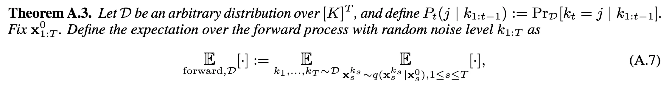
In fact, all I did was translate the concept from the DF paper to the other methods.

$E_{backward}$ is the expectation over the backward process. This backward process is when the model partially denoises frames. The model starts with noisy latents and generates samples by denoising them to various noise levels (or completely to clean frames).

Both are ways to generate noisy latents, they just differ in whether it’s from the model distribution or data distribution

They are a way to measure distance between distributions.

I highly recommend watching this video to understand the KL divergence. This blog also seems to have good intuitions for what it is.

KL divergence is directional, so it is common to see:

$\mathrm{KL}(p_{data} \parallel p_{\text{model}}) \neq \mathrm{KL}(p_{model} \parallel p_{\text{data}})$

The first is the forward KL. The second is the reverse KL.

If two distributions are identical the KL divergence is 0. This is important because if every method is minimizing a combination of KLs, the most optimal model for each method creates the same distribution. In general, divergence measures are 0 if two distributions are identical.

When you think of video generation, some things that come to mind may be Sora2 or Veo3. These are called bidirectional Video generators. They denoise a preset number of frames into a fixed time-length video by denoising every frame at the exact same time. This is a very straightforward way you could imagine just porting over how you train image diffusion models but just doing multiple images at the same time.

If industry is already creating coherent meme videos with the bidirectional method, why do we need another method? Can’t we just press the scale compute button and fix all our problems in video generation?

Here are some problems:

• You can only generate a fixed length video
• You can not stream the video as it is being generated: you have to wait until the whole thing has been made before starting to watch the clip
• You can’t interact with the video as it is being generated (imagine being able to press different arrow keys to make the camera angle of the video move)
• Causality should flow forward in time but bidirectional models let past frames depend on future frames (This is more of a theoretical/philosophical complaint)

Some things that need these capabilities are:

• World models (simulating the world to train other AI policies like robots)
• Low latency video generation (Just like youtube plays your video before it fully loads)
• variable length video generation
• Chain of thought using images (This is an emerging field but perhaps models can think better for some things using images)

Autoregressive video generation (AR video gen) addresses attempts to solve all of the above problems while still having high quality and fast generation of videos.

The first AR video gen method we may think of could be inspired by the LLM field. In the LLM field, the transformer decoder architecture with a causal mask has been used to predict the next language token given the previous language token. If we steal this idea we can come up with the following: predict the next image frame given the previous video frames.

If we implement this idea, we would give our models some context frames from our video dataset and then present it with a frame with gaussian noise and ask it to predict the denoised version.

But as we learned from diffusion and variational autoencoders, asking the model to predict the clean image given noise in one step leads to blurry images. So we can use the idea of decreasing noise levels from image generation to add some amount of noise to the last frame and predict the clean frame.

This is called teacher forcing. The definition of teacher forcing is predicting a continuation of the sequence given ground truth (teacher) frames as conditioning. This is exactly how LLM pretraining is done.

The astute reader may notice the training with teacher forcing for video has trouble in parallelization compared to language modeling. Teacher forcing in language with transformers can just have an upper triangular binary causal mask to train O(N) examples at the same time. (e.g. “The cat in the hat” snippet with one forward pass would predict The -> cat, The cat -> in, The cat in -> the, The cat in the -> hat)

But for video generation we denoise with different levels of noise. So our context will be full of partially noised video frames if we tried to parallelize our training naively.

This can be overcome with a special attention mask where we have the ground truth frames first, then concatenate frames with varying amount of noise after and having a special teacher forcing attention mask:

The goal here is to let every noise frame look at all previous clean frames only and not look at previous noisy frames.

With this attention fix we are able to train our teacher forcing video generation model by combining ideas from both LLMs and image diffusion.

But we have two problems:

• Our attention mask seems more complicated than it needs to be (our attention mask is roughly 4 times bigger than a simple causal mask)
• As we roll out our video using this model, we find that the quality of frames gets bad very quickly the longer we generate for

The reason for the second point is exposure bias:

Exposure bias

#

Exposure bias is when a model is trained on ground-truth data, but at inference time it must rely on its own predictions as input. This is a problem because errors can accumulate over time and the past frames we condition on look nothing like any video the model was trained on so the model is out of distribution.

This is also true for language models, but the space of language is much more compressed than images, and so just brute force training on massive data seems to have brought almost all language context into distribution. To see exposure bias yourself try out [youaretheassistantnow.com] to see how fast you can break the language model with out of distribution context. The website swaps the role of the User and Assistant, so acting very different than a “helpful assistant” to the models queries reveals how exposure bias can break autoregressive generation by taking the context out of training distribution.

A way we could kill two birds with one stone is to allow different noise levels in our history.

First, our attention mask can be the simple binary causal attention mask from language modeling or no mask at all. This is because our context can consist of frames at independent random noise levels, so we no longer have to hide the noisy past frames we want to train in parallel from each other. Noise serves as a continuous mask with no noise being no mask and pure noise being a complete mask.

Second, our model trains on random levels of noise injected into our history, which we can set at test time to have a bit of noise (maybe add a bit of noise to each frame the model generates before feeding it back to the model). This brings the distributions of the history when using self generated frames vs ground truth frames closer (helping exposure bias).

This means we can inject a little bit of noise to our past frames when generating videos to help keep our self generated video (self rollout) in distribution.

As a bonus we unlock different denoising strategies at inference time, which reveal that teacher forcing and bidirectional video generation is actually a subset of diffusion forcing.

Teacher forcing = setting all context frames to no noise and sequentially denoising the last frame Bidirectional video generation = setting all frames to full noise and then denoising all frames in lockstep.

We also unlock a strategy to tradeoff denoising timesteps and latency: We can have a monotonically decreasing noise level. Lets say we do a context length of 5 frames and have noise levels of [0, 0.25, 0.5, 0.75, 1]. We can do an inference step and then slide our window forward by 1 frame. This allows us to produce 1 frame per function evaluation.

The larger the context length we go from 0 noise to 1 noise level ([0, 0.5, 1] vs [0, 0.2, 0.4, 0.6, 0.8, 1]), the more frames it takes for a user conditioning input (such as an arrow key press) to cause a change in a generated frame, but allows the model to use more denoising steps to create higher quality videos.

So cascading noise inference allows us to keep throughput high, while trading off latency and denoising steps. Naturally, this leads us to want to reduce the number of denoising steps to get latency down as much as possible! If we get to one-step denoising our cascading noise inference reduces to teacher forcing inference (Note even if the inference method is the same as teacher forcing here, our training method is different!)

It seems like we found a unifying representation to encompass many of the video generation training methods so far, but we still have some challenges:

• We still haven’t solved the root cause of exposure bias, leading to our generated videos still degrading in quality over time (although it seems to slow down the degradation)
• Our compute requirements grow as $O(N^2)$ with the length of our video, making long video generation a challenge and often leading to videos not consistent over long time periods.
• We need to explore distillation for video generation so we can improve our latency (we want our world models to be as reactive as possible to our inputs)

The first exposure bias problem is tackled by a new training method called self forcing. The second distillation problem is tackled by causvid. The third long term consistency is problem is tackled by rolling forcing.

All of these have issues of their own and do not fully solve the problem they set out to address yet. I write about each below so feel free to skip around depending on which problem you are interested in.

To solve exposure bias you might think of the following: If having self generated frames at inference time is causing exposure bias, why don’t we have self-generated frames during training to get rid of this?

To do this you would generate frames from the model, and then evaluate the generated video as a whole with a loss to tell the model how to nudge the video towards something that has a higher likelihood under the real data distribution.

But a big problem is what loss to use. Since the model generates a sample video from its distribution, we don’t have the corresponding ground truth video from the real data distribution we can just take an L2 loss with.

Consider this example to make the problem more clear: *You decide to become an animator, and want to create animations like those stickfigure fighting videos on youtube.

You decide to improve by drawing some animations yourself. But how do you know exactly how to improve your animation? There is no ground truth version of the animation you created you can compare it to. Maybe you can look through the channel for something similar to what you drew, but you will never find an exact ground truth corresponding to what you drew. So a simple L2 loss is impossible because you can not find the ground truth version of what you made. You need a holistic loss, maybe one that compares the distribution of animations you create vs the ones on the youtube channel and gives you a gradient*

Self forcing solves this by using 3 different distribution level losses (DMD, SiD, GAN).

We go into detail about these losses below.

The main takeaway is that self forcing (SF) does self-rollout (generating frames from scratch) to eliminate exposure bias.

“our training objective matches the holistic distribution of the entire video sequence to the data distribution. In contrast, TF/DF can be understood as performing frame-wise distribution matching” - Self Forcing paper But we show in this blog post that the connection goes much deeper than that.

L2 loss (mean squared error) is the workhorse of diffusion models. The idea is simple: you have a ground truth video $x_0$ from your dataset, you add some noise to get $x_t$, and then you ask your model to predict what the clean video looks like. The L2 loss measures how far off the model’s prediction $\hat{x}_0$ is from the actual clean video:

This works great when you have the ground truth $x_0$ to compare against. This is why L2 pairs naturally with teacher forcing (TF), diffusion forcing (DF), and bidirectional training (BiD) - in all these methods, you start with real data from your dataset and corrupt it with noise. You always know what the “right answer” is.

The magic is that minimizing L2 loss in this diffusion setup is equivalent to minimizing the forward KL divergence $\mathrm{KL}(p_{data} \parallel p_{model})$ assuming gaussian diffusion, which we show in the sections below.

GAN (Generative Adversarial Network) loss is a loss you can use when you don’t have ground truth to compare against. This is the situation in self forcing: your model generates a video from scratch, and there’s no corresponding “correct” video in your dataset to take an L2 loss with.

The GAN solution is clever: instead of comparing your generated video to a specific ground truth, you train a discriminator network to distinguish between “real” videos from your dataset and “fake” videos from your generator. The discriminator learns to spot the difference, while the generator learns to fool the discriminator.

The loss has two parts:

• Discriminator loss: Correctly classify real vs fake videos
• Generator loss: Fool the discriminator (make your generated videos indistinguishable from real)

The original GAN paper proves that with optimal training, this adversarial game minimizes the Jensen-Shannon divergence $\mathrm{JSD}(p_{data} \parallel p_{model})$. The JSD is defined as:

where $M = \frac{1}{2}(p_{data} + p_{model})$ is the mixture distribution (the average of the two distributions). Unlike simply combining forward and reverse KL, JSD measures how far each distribution is from their midpoint, making it symmetric and bounded.

In our video generation context, we use Diffusion-GAN’s trick of discriminating at random noise levels rather than just clean videos. This gives the generator learning signals across the entire denoising trajectory, resulting in the expectation of JSD over noise:

$E_{noise} \big[ \mathrm{JSD}(p_{data} \parallel p_{\text{model}}) \big]$

DMD (Distribution Matching Distillation) loss is like the “reverse” version of L2 loss. While L2 works when you have ground truth to compare against, DMD works when you’re doing self rollout and generating videos from scratch - exactly the situation in self forcing.

The key idea is simple: train two diffusion models to estimate score functions:

• $s_{real}$: a diffusion model trained on real videos from your dataset
• $s_{fake}$: a diffusion model trained on fake videos generated by your model

Then use the difference between these scores as your learning signal:

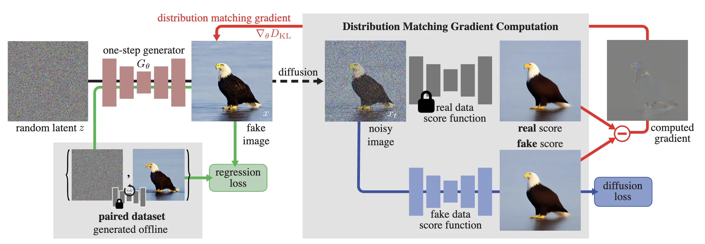
▶ Why does this work?

The DMD paper 3.2 shows this difference approximates the gradient of $\mathrm{KL} (p_{fake} \parallel p_{real})$ - the reverse KL divergence. Intuitively, $s_{real}$ tells you “how to make this video more realistic” and $s_{fake}$ tells you “how to make this video more fake”. The difference nudges your generator away from fake and toward real. If you train $s_{fake}$ on your current generator outputs often, it will be a very good approximator of your generators scores. The reason why we cant just use the generators score directly is because our generator is a one (or few) step model so we cant query the score at an intermediate noise level.

Just like with GANs, we evaluate this at random noise levels across the denoising trajectory, giving us the expected reverse KL over noise levels:

$$E_{backward} \Big[ \mathrm{KL}(p_{fake} \parallel p_{real}) \Big]$$

The reason why we want to evaluate the loss at different noise levels is because for example if our generator is randomly initialized, our p_model will have very little overlap with p_data and so the scores are not well defined almost everywhere. (an intuitive example would be paintings by me vs by Van Gogh would look much more similar if we add a bunch of noise to them :) )

This makes DMD the natural pair for self forcing: SF handles the sampling (generating from scratch), while DMD handles the loss (learning without ground truth). Together they optimize reverse KL, which we show in detail below.

The explicit gradient formula for DMD (from DMD page 5) is:

where $w_t$ and $\alpha_t$ are weighting terms that depend on the noise schedule, and $G$ is the generator network.

In the training algorithm presented in the Self Forcing paper, they sample a scalar timestep that is the same across frames, but in the actual code they sample independent timesteps per frame. This is an important distinction because if each frame didn’t have their own timestep like the concept in diffusion forcing, our autoregressive inference algorithm would always be out of distribution—the context frames would always be clean regardless of the denoising timestep for the very last frame we are denoising.

This notational inconsistency could be easily fixed by moving the timestep sampling inside the first for loop.

We saw that DF is to L2 loss as SF is to DMD loss. DMD is like the “reverse” version of L2, useful when you don’t have the ground truth available because your generator is doing self rollout to generate data during training.

When you combine DF and DMD, you get something that is a hybrid between reverse and forward KL. Causvid explores this and presents it as a distillation method. However, in the code, the justification for using the DF framework and using the forward process to generate noisy samples from the ground truth data distribution is that it is an approximation to generating samples from self rollout citing DMD2 section 4.5. So unapproximated Causvid is self forcing. If you use self rollout to generate samples and use DMD, we established in SF+DMD that this is optimizing the reverse KL divergence. The option to use the approximation or not is in the causvid code here and the approximation is enabled for the causal distillation presented in the paper

Ok, but is the approximated Causvid which is DF+DMD representable by a linear combination of forward and reverse KL? The answer is no.

DMD is minimizing the reverse KL between p_data and p_model. This is because we are marginalizing over the model distribution and calculating the difference in scores. But DF+DMD messes with the distribution we are marginalizing over because samples are created by picking a random timestep and then doing the forward process to that step and then a backward process. Mathematically this is writable as a pushthrough distribution but is not equal to either p_data, p_model, or a linear combination of the two. The detailed proof is in the appendix.

Conclusion: Causvid without the self rollout approximation is algorithmically identical to SF+DMD. Causvid with self rollout approximation is DF+DMD and is not representable as a simple linear combination of forward and reverse KL divergences. I have yet to prove if this can be represented as an f-divergence.