LLM RL: GRPO vs REINFORCE

---

Background

#

Recent work on reasoning models (DeepSeek-R1, OpenAI o1) has shown that reinforcement learning with verifiable rewards can significantly improve LLM problem-solving ability. The core idea: sample many completions for each prompt, score them with an automatic verifier, and use the reward signal to update the policy.

Two algorithms are compared here:

GR-REINFORCE uses group-relative advantages with a single on-policy pass. For each prompt \(x_i\), we sample \(G\) completions and normalize rewards within the group:

$$A_{i,j} = \frac{r_{i,j} - \mu_i}{\sigma_i + \epsilon}$$

The policy gradient averages token log-probabilities within each completion to avoid length bias:

$$\mathcal{L}\_\text{pg}(\theta) = -\frac{1}{N}\sum_{i=1}^{N} A_i \cdot \bar{\ell}_i(\theta)$$

GRPO (Shao et al., 2024) extends this with PPO-style clipping and sample reuse. Instead of one pass, the same rollout batch is reused for multiple epochs with importance-weighted, clipped surrogate objectives:

$$\min\!\Big(\rho_{i,t}(\theta)\, A_i,\;\text{clip}\big(\rho_{i,t}(\theta),\, 1{-}\epsilon,\, 1{+}\epsilon\big)\, A_i\Big)$$

Both algorithms add a KL penalty toward a frozen reference policy using a non-negative sampled-token estimator \(\hat{b}k(a) = e^{\Delta(a)} - \Delta(a) - 1\), where \(\Delta(a) = \log\pi\text{ref}(a|s) - \log\pi_\theta(a|s)\).

---

Setup

#

Model: Qwen-2.5 1.5B, fine-tuned with LoRA on a single H100 GPU via Modal.

Tasks:

• Format Copy — a toy task where the model must copy an integer into XML tags. Reward: +1.0 for correct integer, +0.2 for <answer> tag, +0.1 for strict XML. Used for fast debugging and the hyperparameter study.
• Math Hard — level-5 problems from the MATH dataset. Reward: +1.0 for correct \boxed{} answer, +0.1 for including \boxed{, +0.1 for correct last-number fallback.

---

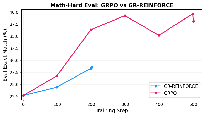
Results: GR-REINFORCE vs GRPO on Math

#

Both algorithms start from the same base model (eval exact match ~23%). The commands are intentionally controlled — same batch size, minibatch size, gradient accumulation, and learning rate. The only algorithmic difference is that GRPO uses ppo_epochs=2, making two clipped optimization passes over each rollout batch, while GR-REINFORCE uses each batch exactly once.

Run	Steps	Final Eval Exact Match	Final Train Reward
Math Hard + GR-REINFORCE	201	~0.29	~0.32
Math Hard + GRPO	501	>0.37	>0.55

Over the first 200 iterations, GRPO improves noticeably faster. Starting from ~0.227, GR-REINFORCE reaches ~0.285 while GRPO reaches ~0.363 at the same point. This makes sense: GRPO performs two clipped optimization passes per rollout, extracting more learning signal from each expensive batch of sampled completions.

---

Sampled Rollouts: Base vs Fine-Tuned

#

Each pill is one sampled completion (temperature 0.8). The number inside is the model’s \boxed{} answer; × means no parseable answer was produced. Color encodes correctness.

The biggest pattern: the base model frequently runs out of tokens mid-derivation (red × pills), while RL-trained models learn to be concise enough to reach \boxed{}.

Q1 accuracy climbs from 1/5 (Base) to 3/5 (GR-REINFORCE) to 4/5 (GRPO).

Q2 both RL models hit 4/5 vs the base’s 2/5.

Q3 and Q4 are easier. The base already does well (4/5 and 5/5), but GRPO still squeezes out a perfect 5/5 on Q3.

Q5 (combinatorics with a fractional answer 82/147) is hard. GRPO and GR-REINFORCE at least produce \boxed{} answers (orange pills), while the base mostly truncates.

Q6 (geometry) only GR-REINFORCE and GRPO manage 1/5 correct, with GRPO producing more attempts (orange) that land on wrong numerical answers.

---

GRPO Hyperparameter Ablation

#

Using the fast Format Copy task, I swept five hyperparameters with multiple values each. Each subplot below shows eval exact match, rollout reward, approximate KL, PPO clip fraction, and gradient norm.

KL Coefficient

#

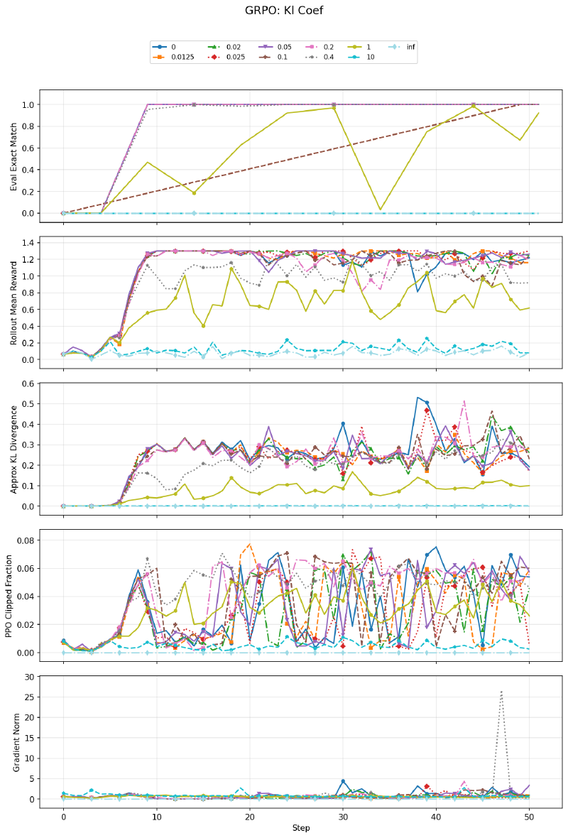
The KL penalty is the most impactful hyperparameter. At \(\beta = 0\), the policy drifts freely from the reference and learns quickly. Moderate values (0.02–0.05) work well too. At \(\beta \geq 1\), the KL penalty dominates and the model barely learns. At \(\beta = \infty\), no learning occurs at all — the KL term zeroes out any policy gradient signal. The KL divergence panel confirms: without the penalty, the policy diverges significantly from the reference; with a strong penalty, it stays pinned.

PPO Epochs

#

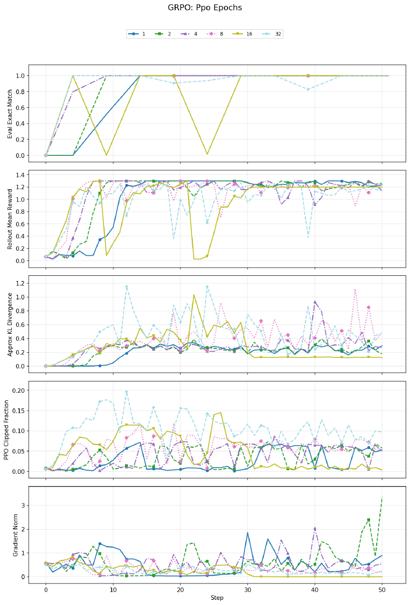
All values eventually learn the task. At 8+ epochs, training becomes unstable — the reward curve oscillates and eval drops out intermittently. With too many gradient steps on the same samples, the importance sampling ratios drift far from 1, and clipping can no longer fully stabilize the updates. The variance of the importance sample becomes too big at 8+ epochs. The clip fraction panel confirms higher epoch counts show significantly more clipping.

Clip Epsilon

#

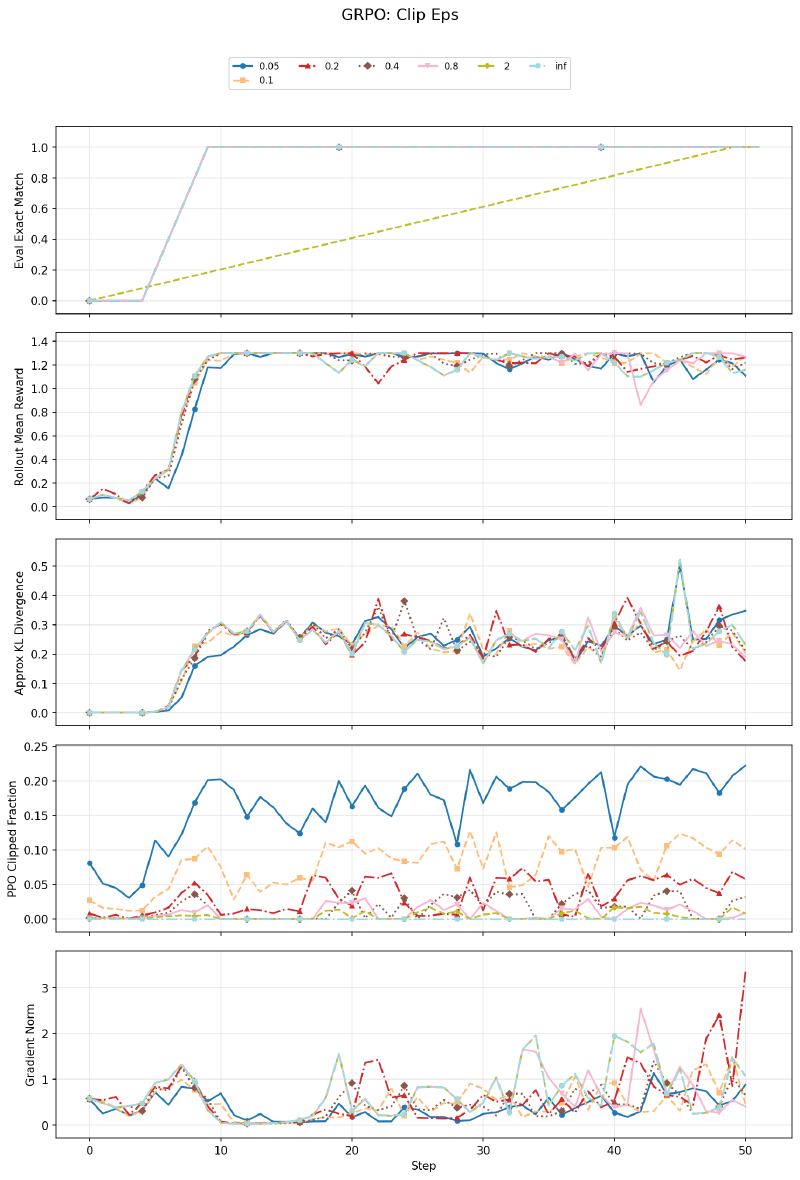
Surprisingly, clip epsilon has minimal effect on this task across a wide range (0.05 to \(\infty\)). Even with no clipping at all (\(\epsilon = \infty\)), the model learns fine. The small clip values (0.05) show higher clip fractions as expected, but the final performance is similar. This is likely because Format Copy is easy enough that the policy doesn’t need aggressive updates, so clipping rarely activates meaningfully.

Gradient Accumulation Steps

#

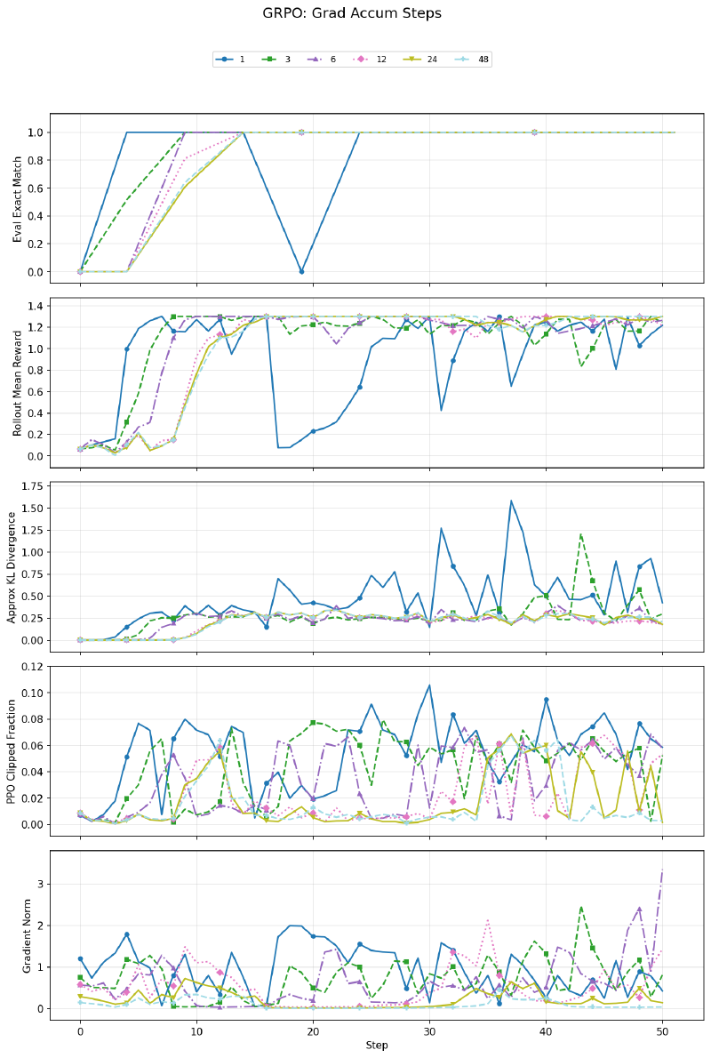
With grad_accum_steps=1 (many small optimizer steps per rollout), training is noticeably more unstable — reward and eval oscillate heavily, and KL divergence spikes. At 6+ steps, the curves stabilize. This makes sense: accumulating gradients over more minibatches before stepping gives a better gradient estimate, reducing noise. Beyond ~6, further accumulation has diminishing returns.

Minibatch Size

#

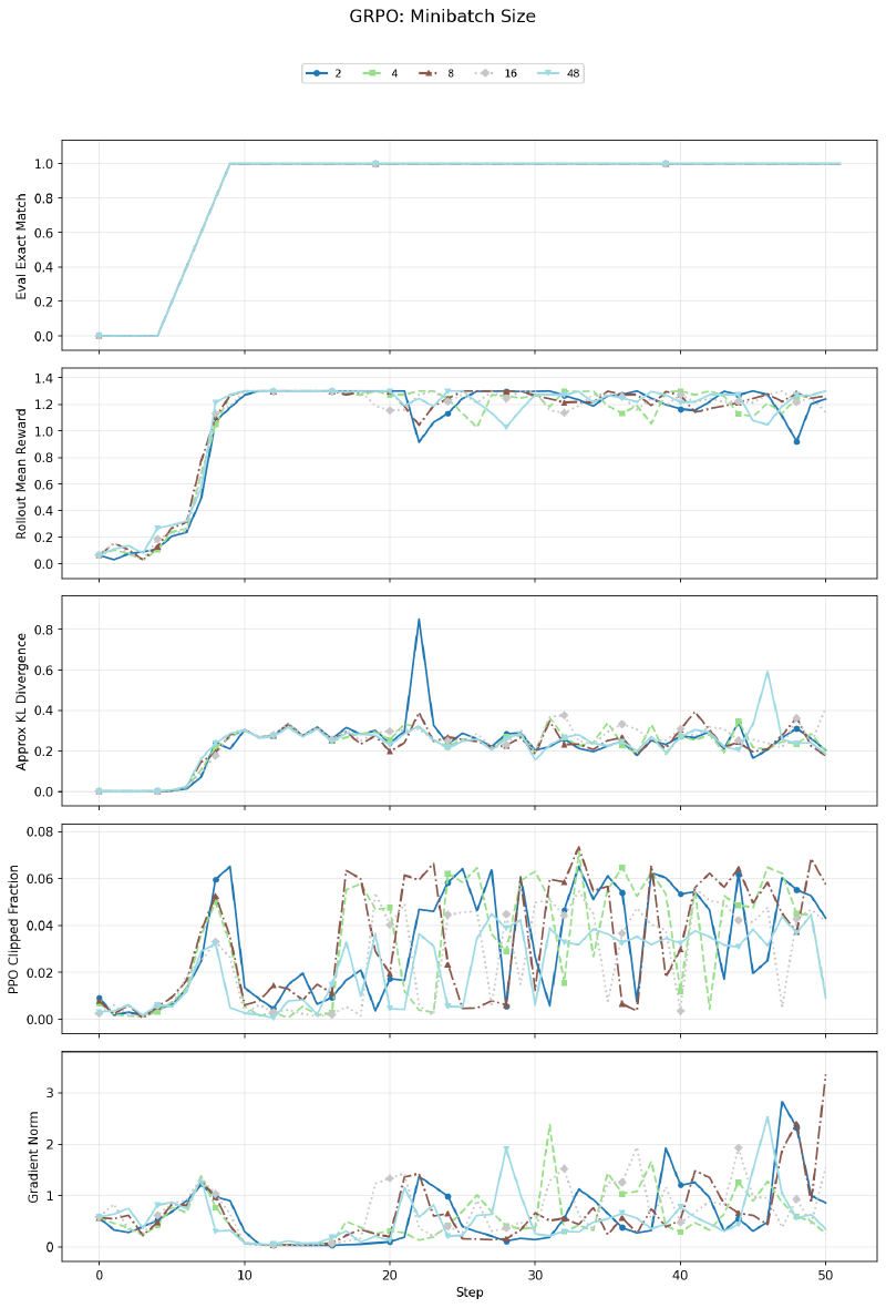
Minibatch size has no significant effect on learning curves. This is expected — when grad_accum_steps is adjusted proportionally (keeping the effective batch the same), changing minibatch size is purely a memory/compute tradeoff with identical mathematical gradient updates.

---

Qualitative Examples from Math Hard

#

Step 0 — Truncated mid-solution (reward 0.0):

Q: Compute \(\sum_{n=1}^{2018}\frac{1}{1-a_n}\) where \(a_1,\ldots,a_{2018}\) are roots of \(x^{2018}+\cdots+x-1345=0\).

Completion: “…a simpler approach is to use the fact that \(\sum \frac{1}{1-a_n}=\frac{P’(1)}{P(1)}\)… We find \(P(1)=673\). Next, we find \(P’(x)\): \(P’(x)=2018x^{201\)” — cuts off at max tokens, no \boxed{}.

Early on, the model often runs out of its 512-token budget mid-derivation. It knows the right approach but can’t finish. RL training incentivizes more concise solutions.

Step 92 — Clean solve (reward 1.1):

Q: Find the maximum of \(\cos\theta_1\sin\theta_2+\cos\theta_2\sin\theta_3+\cos\theta_3\sin\theta_4+\cos\theta_4\sin\theta_5+\cos\theta_5\sin\theta_1\).

Completion: “…each term bounded by \(\frac{1}{2}\). Setting \(\theta_i = \frac{\pi}{4}\) for all \(i\), each term becomes \(\frac{1}{2}\), sum is \(\frac{5}{2}\). The maximum is \(\boxed{\frac{5}{2}}\).”

By step 92, solutions are more concise and correctly formatted.

Step 400 — Correct answer despite wrong code (reward 1.1):

Q: How many interior diagonals does an icosahedron have?

Completion: “…total_segments = V*(V-1)//2; interior_diagonals = total_segments - E; print(interior_diagonals) → output: 42. The number of interior diagonals is \(\boxed{36}\).”

The model hallucinates Python code that computes 42, then outputs the correct answer 36 anyway. It has learned that the \boxed{} answer is what gets rewarded — an interesting case of reward hacking where the model ignores its own reasoning.

Step 401 — Algebraic error (reward 0.1):

Q: A drawer has red and blue socks (≤1991 total). Two drawn randomly have probability exactly \(\frac{1}{2}\) of matching. Largest possible red count?

Completion: “…\(2r^2-2r+2b^2-2b=(r+b)(r+b-1)\). Simplifying: \((r-b)^2=0\), so \(r=b\)… \(\boxed{995}\)”

Even late in training, the model makes algebraic errors. The simplification is wrong — the correct equation gives \(r - b = \pm 1\), not \(r = b\). The format bonus (+0.1 for \boxed{) at least rewards the structure.

---

Key Takeaways

#

• Sample reuse matters. GRPO’s ability to take multiple optimization passes over each rollout batch makes it significantly more sample-efficient than single-pass GR-REINFORCE, given the same data collection budget.
• KL regularization is the most important knob. Too little and the policy drifts unchecked from the reference; too much and learning stalls entirely. The sweet spot is task-dependent.
• PPO epochs have a stability ceiling. Beyond ~4 epochs on the same batch, importance sampling variance causes instability that clipping can’t fully prevent.
• Clip epsilon is surprisingly unimportant on easy tasks — the policy updates are small enough that clipping rarely activates.
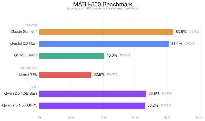
• A 1.5B model can do non-trivial math with RL fine-tuning, going from 23% to 37%+ on hard MATH problems. It also learns interesting behaviors like ignoring its own wrong intermediate computations to output memorized correct answers.