Offline RL: SAC+BC, IQL, and Flow Q-Learning

---

Background

#

In offline RL we’re given a fixed dataset \(\mathcal{D}\) of transitions \((s, a, r, s’)\) sampled from some behavior policy \(\pi_\beta\), and asked to learn a good policy without collecting any new data. The central difficulty is distributional shift: a naive actor-critic trained on \(\mathcal{D}\) will happily query \(Q(s, a)\) at out-of-distribution actions where the network is free to hallucinate large values, and the policy will then chase those phantom rewards.

All three algorithms in this post are different ways to stop that from happening.

I evaluate them on two tasks from OGBench:

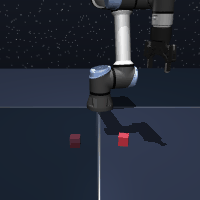
• cube-single-play-singletask-task1-v0 — pick-and-place a cube with a robot arm. Short horizon, fairly unimodal behavior data.
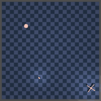
• antsoccer-arena-navigate-singletask-task1-v0 — an ant morphology pushing a ball to a goal. Long horizon, much more multimodal.

Both tasks use sparse rewards (-1 every step, 0 on success) and continuous bounded action spaces. Concretely:

cube-single (Franka arm + one block on a table):

• Observation \(s \in \mathbb{R}^{28}\): 6 joint angles + 6 joint velocities + 3 end-effector position (recentred on the workspace and rescaled ×10) + \((\cos\theta, \sin\theta)\) for the end-effector yaw + gripper opening + gripper contact flag + 3-d block position (same recentring) + 4-d block quaternion + \((\cos, \sin)\) of the block yaw. That is: the robot’s proprioceptive state plus the block’s pose, nothing else.
• Action \(a \in [-1, 1]^{5}\): 3-d end-effector delta + wrist-yaw delta + gripper open/close.
• Horizon 200 steps.

antsoccer-arena (quadruped ant pushing a ball through a maze):

• Observation \(s \in \mathbb{R}^{42}\): the MuJoCo qpos (22) and qvel (20), concatenated. This includes the ant’s global \(xy\), trunk orientation quaternion, 8 leg joint angles, the ball’s 3-d position and quaternion, and all of their velocities. Again: just the raw physical state.
• Action \(a \in [-1, 1]^{8}\): torques for the ant’s 8 leg actuators (2 per leg × 4 legs).
• Horizon 1000 steps.

With \(\gamma = 0.99\) and rewards in \({-1, 0}\), the value function should stay bounded in \([-1/(1-\gamma), 0] = [-100, 0]\).

---

Part 1: SAC+BC

#

Algorithm

#

SAC+BC is the simplest way to make an off-policy actor-critic behave in the offline setting: just add a behavioral cloning term to the SAC actor loss. Two Q-networks and a Gaussian policy are trained with:

$$\mathcal{L}(Q) = \sum_{i=1}^{2} \mathbb{E}_\mathcal{D}\Big[\big(Q_i(s, a) - y\big)^2\Big], \quad y = r + \gamma\, \tfrac{1}{2}\sum_{j=1}^{2} \bar{Q}_j(s', a'),\ a' \sim \pi(\cdot|s')$$$$\mathcal{L}(\pi) = \mathbb{E}_\mathcal{D}\!\Big[ -\tfrac{1}{2}\sum_i Q_i(s, a_\pi) + \tfrac{\alpha}{|\mathcal{A}|}\|a - a_\pi\|_2^2 + \beta \log \pi(a_\pi|s) \Big]$$

Two small tweaks from vanilla SAC that matter for offline: (1) drop the entropy term in the Bellman backup, and (2) use the mean of the two target \(Q\)’s rather than the min. Entropy is still automatically tuned for the actor but doesn’t leak into value targets.

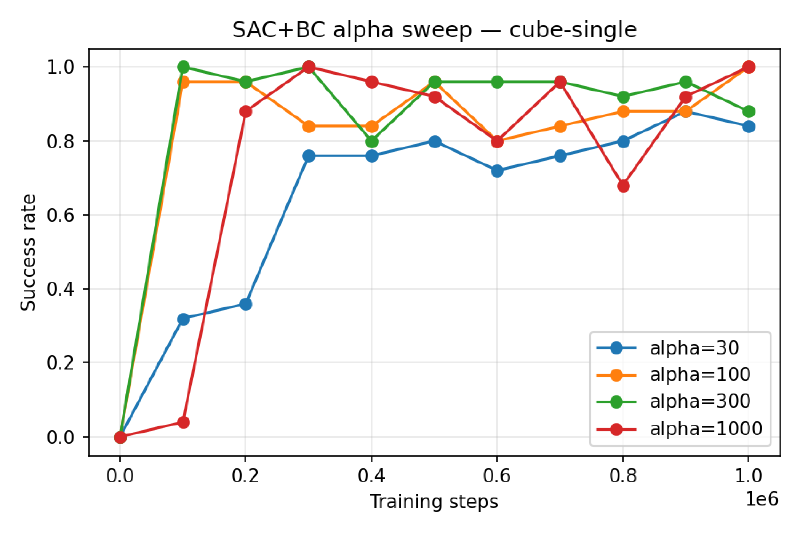
The BC coefficient \(\alpha\) is the knob. Large \(\alpha\) keeps the policy on-distribution; small \(\alpha\) lets it chase Q but risks OOD exploitation.

Best runs

#

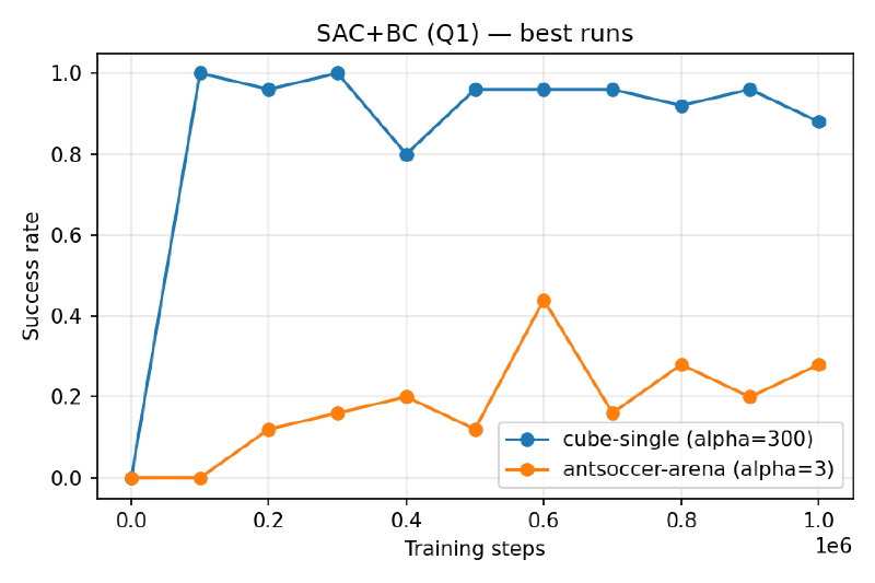
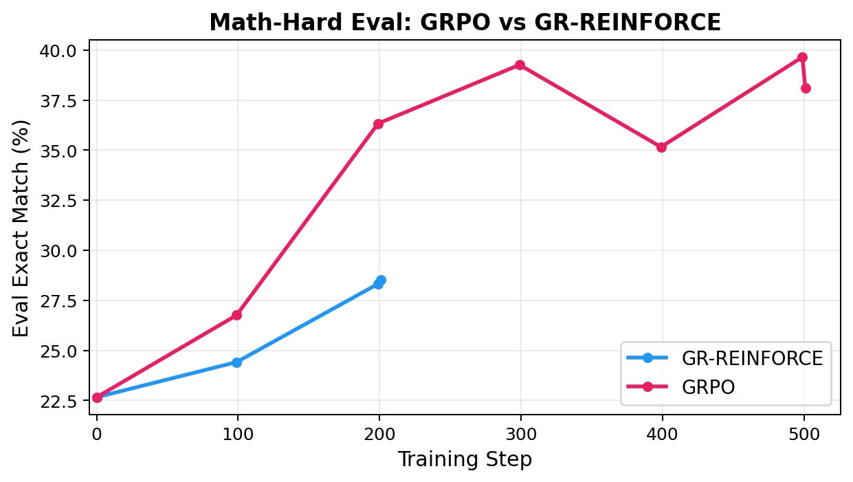
α sweep on cube-single

#

---

Part 2: Implicit Q-Learning (IQL)

#

Algorithm

#

IQL avoids querying \(Q\) at OOD actions at all. Instead of a Bellman optimality backup, it trains a value function \(V(s)\) to estimate the upper expectile of \(Q(s, \cdot)\) over in-dataset actions:

$$\mathcal{L}(V) = \mathbb{E}_\mathcal{D}\Big[ \ell_2^\tau\big(V(s) - \min_{i}\bar{Q}_i(s, a)\big) \Big], \quad \ell_2^\tau(x) = |\tau - \mathbb{I}(x > 0)|\, x^2$$

Expectile loss with \(\tau \to 1\) makes \(V\) track the max over actions that are supported in the dataset. Then the Q backup uses this \(V\):

$$\mathcal{L}(Q) = \sum_i \mathbb{E}_\mathcal{D}\big[(Q_i(s, a) - r - \gamma V(s'))^2\big]$$

Finally, the policy is extracted via advantage-weighted regression — weighted behavioral cloning where high-advantage actions get large weights:

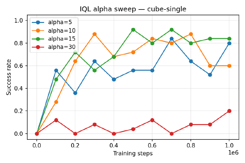
$$\mathcal{L}(\pi) = \mathbb{E}_\mathcal{D}\Big[ -\min\!\big(e^{\alpha A(s, a)},\, M\big)\, \log \pi(a|s) \Big], \quad A(s, a) = \min_i Q_i(s, a) - V(s)$$

No OOD queries anywhere. I fixed \(\tau = 0.9\) and tuned \(\alpha \in {5, 10, 15, 30}\).

Best runs

#

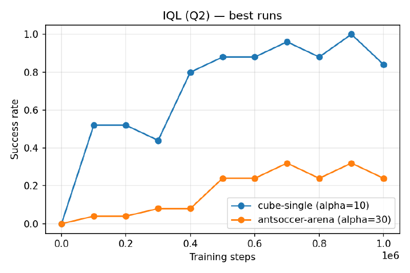
α sweep on cube-single

#

SAC+BC vs IQL

#

Both hit 1.00 peak performance on cube-single, and similar peak performance on antsoccer-arena. SAC+BC’s viable α spans two orders of magnitude ({30, 100, 300, 1000}) while IQL only tolerates a tight band near α=5–15 — past α=30 it collapses. So SAC+BC seems like the more forgiving method. –>

---

Part 3: Flow Q-Learning (FQL)

#

Motivation: why not just use a flow policy in SAC+BC?

#

The natural extension of SAC+BC to flow policies is FBRAC: replace the squared BC loss with a flow-matching loss and keep the rest. The flow policy is an ODE integration of a vector field \(v(s, \tilde a, t)\) from \(t=0\) (Gaussian noise) to \(t=1\) (actions):

$$\pi_v(s, z) = \text{ODESolve}\big(v(s, \cdot, t);\, z,\, t\!=\![0,1]\big)$$

Training the actor requires \(\partial Q(s, \pi_v(s, z)) / \partial v\), which means backpropagating through the ODE solver — a multiply of ~(layers × integration steps) Jacobians. Unstable and expensive.

FQL: add a one-step policy

#

FQL sidesteps the BPTT by training an additional feedforward one-step policy \(\pi_\omega(s, z)\) that maps noise directly to actions in one network call. Three networks:

1. $$\mathcal{L}(v) = \mathbb{E}\Big[\tfrac{1}{|\mathcal{A}|}\|v(s, \tilde a, t) - (a - z)\|_2^2\Big], \quad \tilde a = (1-t) z + t\, a$$
2. $$y = r + \gamma\,\tfrac{1}{2}\sum_j \bar Q_j(s', \pi_\omega(s', z))$$
3. $$\mathcal{L}(\pi_\omega) = \mathbb{E}\Big[ -\tfrac{1}{2}\sum_i Q_i(s, \pi_\omega(s, z)) + \tfrac{\alpha}{|\mathcal{A}|}\|\pi_\omega(s, z) - \pi_v(s, z)\|_2^2 \Big]$$

The distillation term replaces the flow-matching term in FBRAC, so the only gradient path through \(\pi_v\) is stopped — no BPTT. The one-step policy is what’s deployed at eval time.

Three implementation details that actually matter: clip flow-policy outputs to \([-1, 1]\) before feeding them to \(Q\); don’t clip \(\pi_\omega\)’s output in the distillation term (otherwise OOB actions have no gradient to come back); and use the mean of target Q’s for antsoccer-arena — the min is too pessimistic on long-horizon tasks.

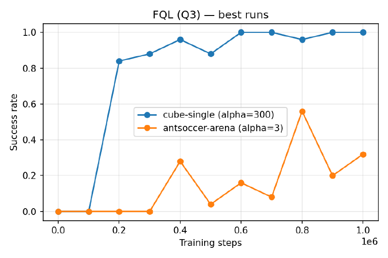
Best runs

#

---

Infrastructure notes

#

I ran all experiments on Modal, four agents in parallel per GPU using the course’s helper script. A single 1M-step FQL run on one NVIDIA A10 GPU took about 5 hours; four in parallel took ~6 hours total, so the α sweeps were essentially free once I had the job template.