Ever wondered how we can turn a bunch of 2D photos into a 3D model? That’s exactly what I explored in this project using Neural Radiance Fields (NeRF). Let me take you through my journey of building one from scratch!

Starting Simple: 2D Image Reconstruction Link to heading

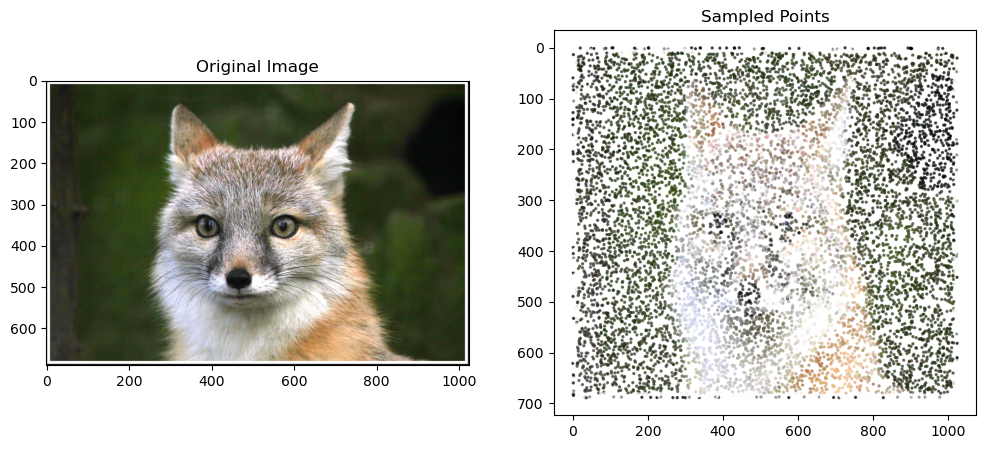
Before diving into the full 3D challenge, I started with a simpler task: reconstructing a 2D image using neural networks. Here’s how it works:

1. The network takes a coordinate (like x=100, y=150) as input
2. It predicts what color should be at that point
3. We repeat this process with 10,000 random points per iteration
4. After 1,000 iterations (that’s 10 million points!), we get a complete image

The Network Architecture Link to heading

For this 2D version, I used a straightforward Multilayer Perceptron (MLP):

Positional encoding translate an intiger into a form more friendly to a neural network to handle. This is usually done by converting the number into a bunch of sin or cos waves.

Here is what a positional encoding looks like. The y axis has increasing numbers (think going from 0 to 1). The one on the left goes from 0 at the top to 1 at the bottom and the one on the right goes from 1 at the top to 0 at the bottom.

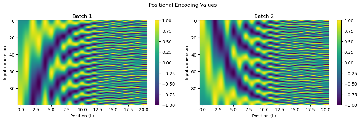
In this project, I set the positioonal encodings to L=10, meaning each 2D point would become a 2 by 21 (because 2 * L + 1 = 21) vector. This is because for positional encoding we do

With the unaltered number at the start, then alternating sin and cos terms.

Experimenting with Different Settings Link to heading

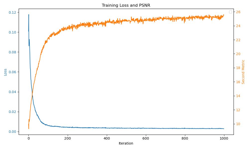
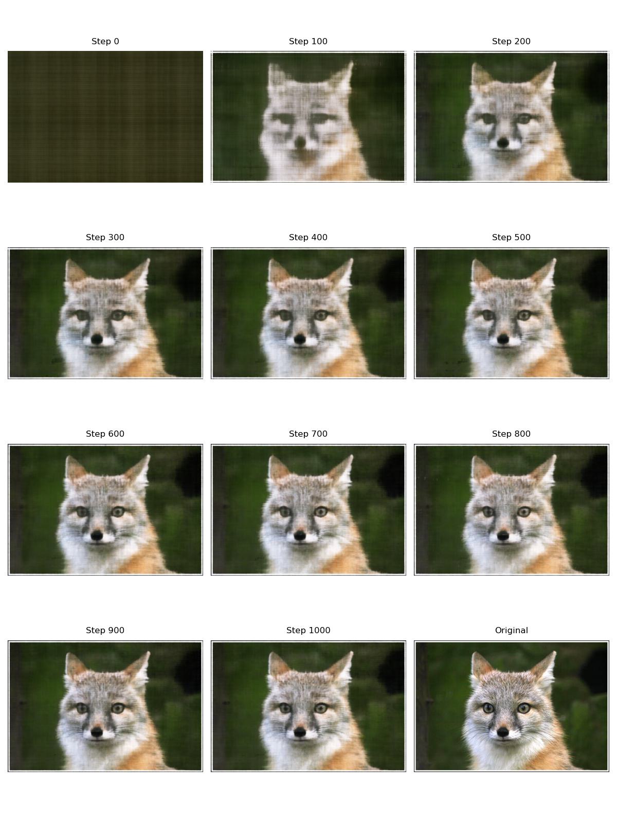
I played around with various network configurations to see how they affected the image quality. Here are the results:

Default Settings (256 hidden layer neurons, 3 hidden layers just like the above picture) Link to heading

Shallow Network (256 hidden layer neurons, 1 hidden layer) Link to heading

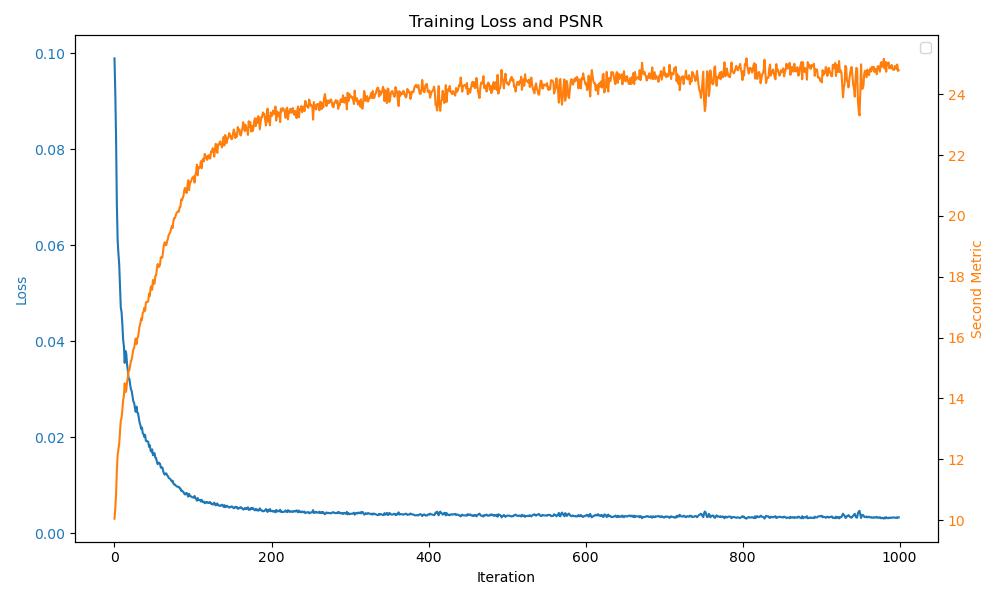
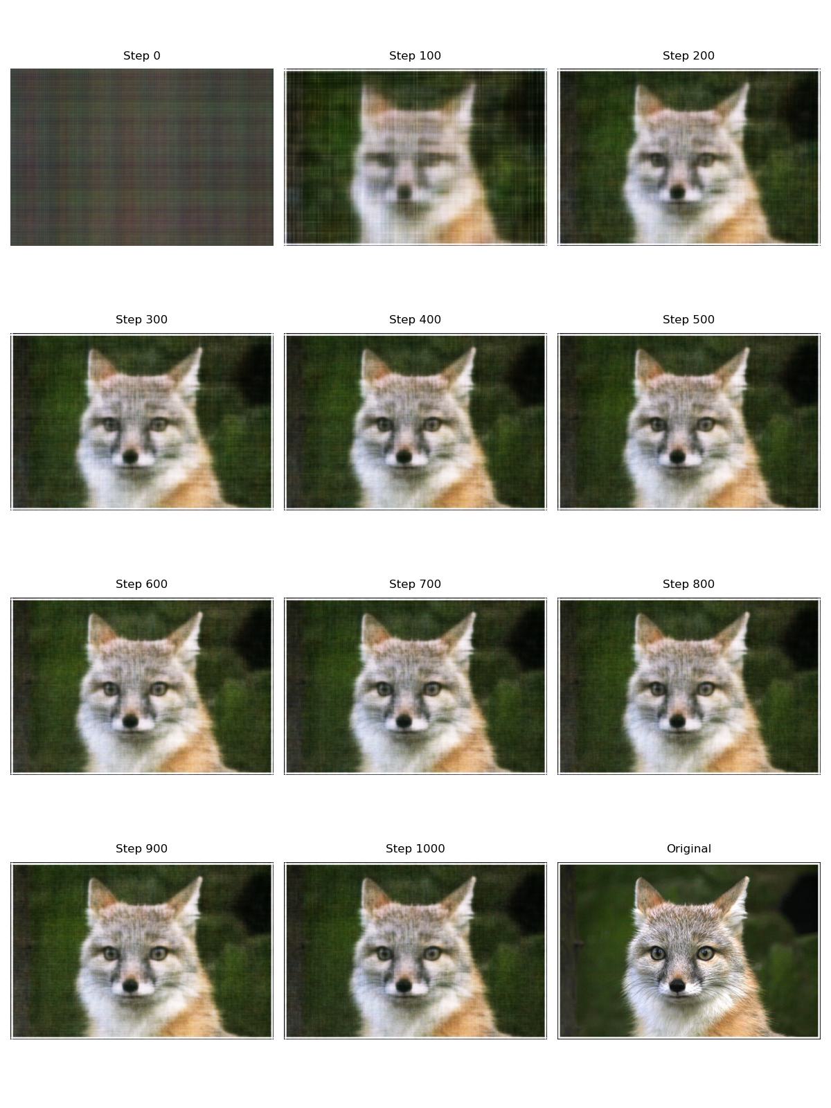
Compared to the default settings, the final image seems to suffer a bit more from black cross shaped artifacts.

Smaller Network (128 hidden layer neurons, 3 hidden layers) Link to heading

Compared to the default settings, the fur seems a bit less detailed with white blurred regions replacing some contrasty areas. There does not seem to be the black cross artifacts that were present in the first experiement with only 1 hidden layer.

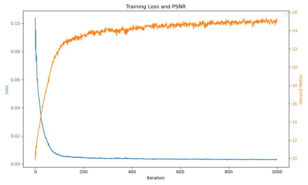
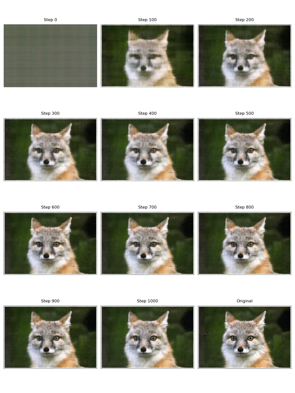
Alpacca (default settings) Link to heading

I tried this with a picture of an alpacca. It seems to work similarly.

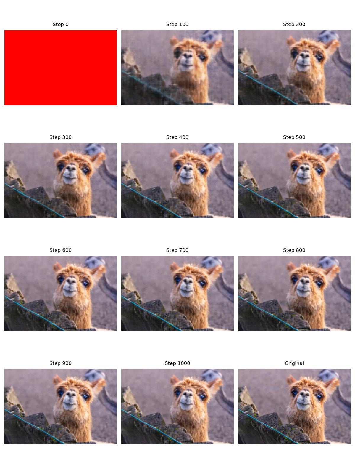
The final rendering seems to be a bit blurred compared ot the original image.

Leveling Up: 3D NeRF Link to heading

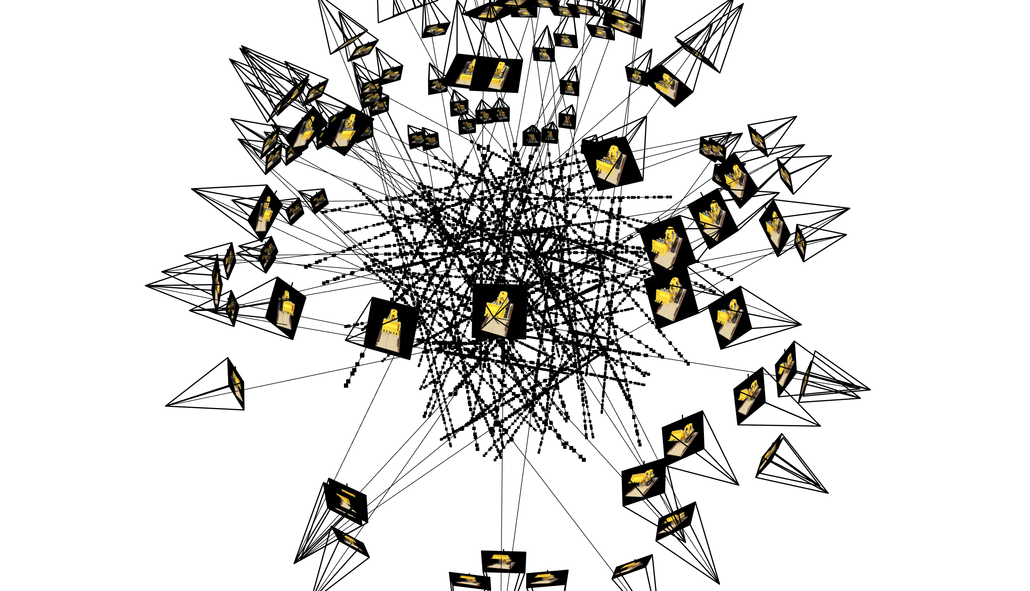
Now for the exciting part - creating a full 3D model from multiple images! The process is similar to the 2D version, but instead of sampling points in a flat image, we shoot rays from each camera and sample points along these rays.

How It Works Link to heading

Here’s a visualization of the ray sampling process that happens at every training step. Each camera shoots rays into the scene, and the model tries to predict the color and density of the points along these rays such that the resulting image is consistant with our training images.

The 3D Architecture Link to heading

The 3D version uses a more sophisticated network architecture to handle the additional complexity:

Results Link to heading

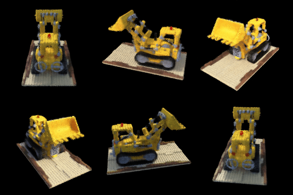
Check out these cool visualizations of the final result:

Distance Field Visualization (PSNR = 26) Link to heading

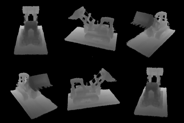
This is achieved by intigrating the distance from the camera over the density instead of intigrating the color over the density.

Final 3D Model (PSNR = 26) Link to heading

Training Progress Link to heading

Watch how the model improves over time in this gif (I sped up the middle):

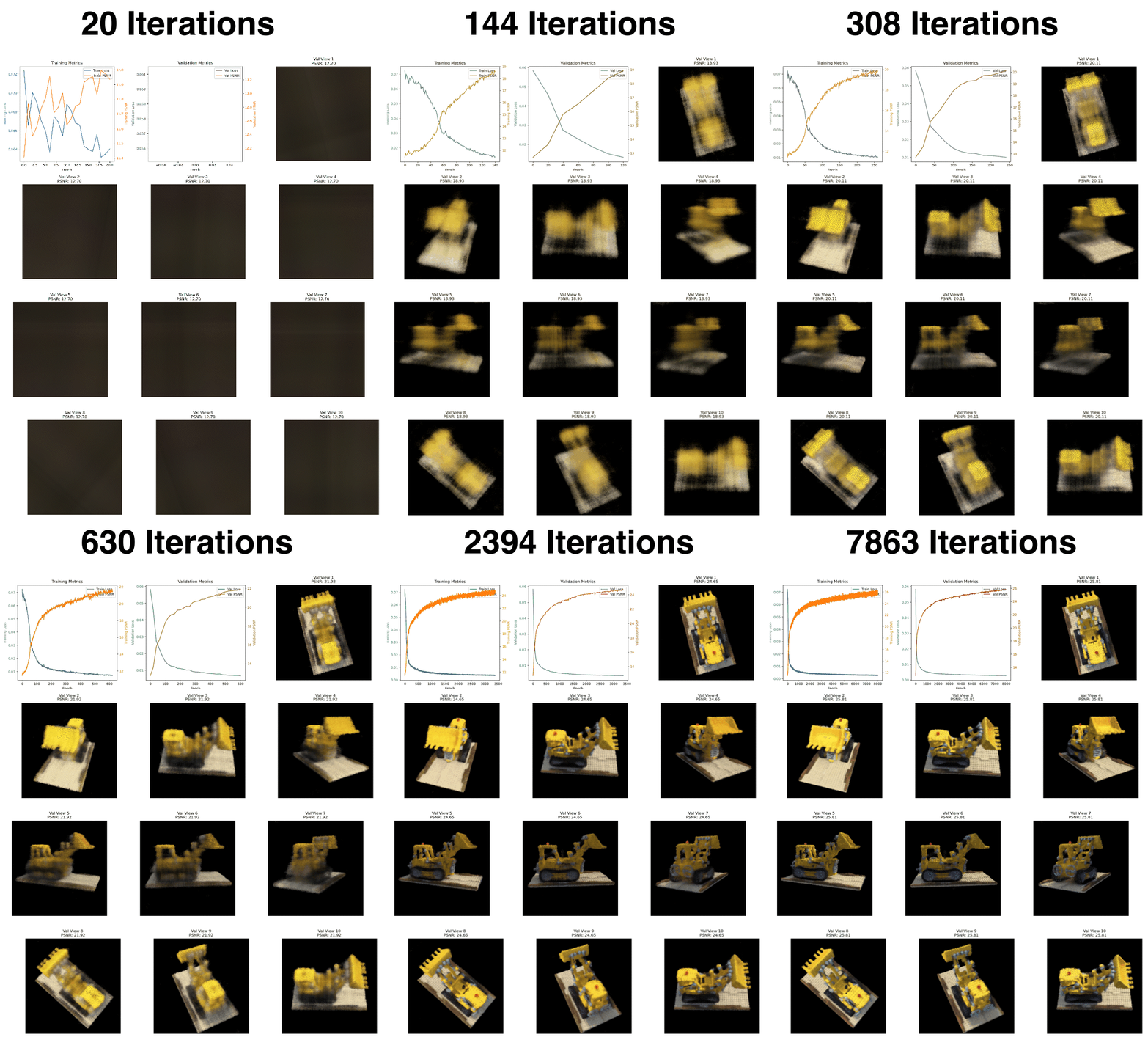
Here are the final views after 8000 iterations from the validation camera perspectives.

Here is the loss and psnr over the 8000 iterations (batch size of 10,000)

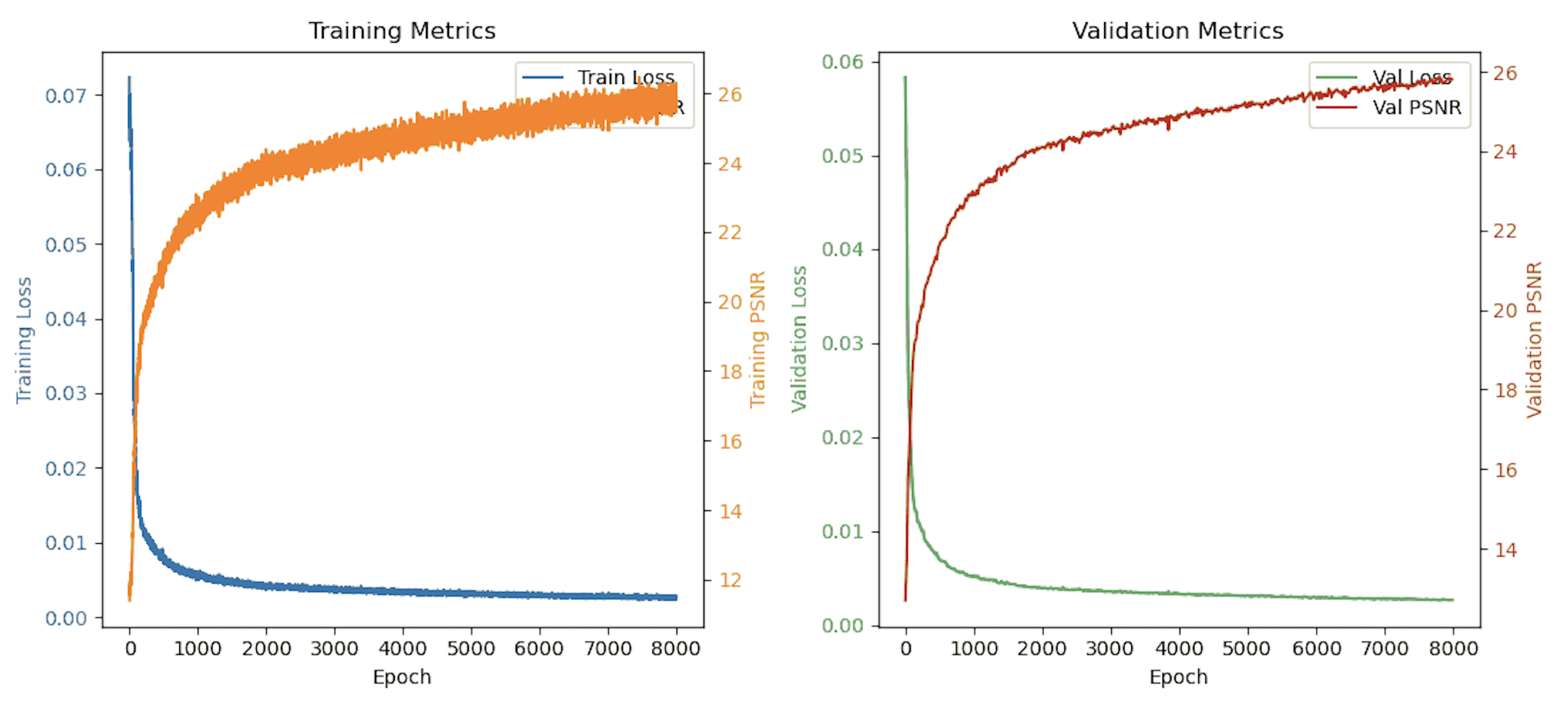
We achieved a validation PSNR just shy of 26!

This project really showed me the power of neural networks in creating 3D content from 2D images. It’s amazing how we can teach a network to understand and recreate 3D space!

Here is the assignment this is based off of

Implementation Details on each part Link to heading

Part 2.1 - Camera and Ray Implementation Link to heading

I implemented three fundamental coordinate transformation functions that form the backbone of my NeRF pipeline:

I created transform(matrices, vectors) to handle coordinate system conversions between camera and world space. This function adds homogeneous coordinates and performs efficient batch matrix multiplication using numpy operations. It was crucial to handle batched inputs correctly here as this function gets called frequently during training.

For pixel_to_camera(K, uv, s), I implemented the conversion from pixel coordinates to camera space. This involved applying the inverse camera intrinsics matrix and properly handling depth scaling. I made sure to support both single and batched inputs using numpy broadcasting for efficiency.

In pixel_to_ray(K, c2w, uv), I combined the above functions to generate rays for each pixel. The function calculates ray origins and normalized directions in world space. Getting the normalization right was important here to ensure proper sampling later in the pipeline.

Part 2.2 - Sampling Link to heading

My sample_along_rays() implementation focuses on efficient point sampling along rays. For the Lego scene, I used near=2.0 and far=6.0 bounds. During training, I added small random perturbations to prevent overfitting to fixed sampling points. This function efficiently handles batched computations using numpy operations.

Part 2.3 - Data Loading Link to heading

I created the RaysData class to integrate everything into a cohesive data pipeline. This class manages images, camera intrinsics, and camera-to-world transforms. It implements efficient ray sampling through the sample_rays() method and handles all the coordinate system conversions needed. I made sure to properly manage memory by implementing batch sampling for training.

Part 2.4 - Neural Network Link to heading

For the NeRF model itself, I implemented a deep MLP with positional encoding for both coordinates (L=10) and view directions (L=4). The network includes skip connections at layer 4 and splits into separate branches for density and color prediction. I used ReLU activation for density (to ensure positive values) and Sigmoid for color (to bound outputs between 0 and 1).

Part 2.5 - Volume Rendering Link to heading

My volume_render() function implements the volume rendering equation using PyTorch operations. It computes alpha values from predicted densities, calculates transmittance using cumulative products, and combines colors using the volume rendering weights. I made sure to handle batched computations efficiently on the GPU and included support for both training and inference modes.

All these components work together in my training loop to optimize the NeRF representation. I save training progress through GIFs showing both the training metrics and novel view synthesis results. The implementation achieves good results on the Lego dataset while maintaining reasonable training times on available GPU resources.