Flow Matching - How Image Generation Works

TLDR: We learn a Neural Network that takes any point from our source distribution and flow it into a sample point from a target distribution. Here we flow from a 2D unit gaussian to a checkboard pattern. In Image generators we would go from a high dimensional unit gaussian to the distribution of images of cats for example.

Introduction to Image Generation
#

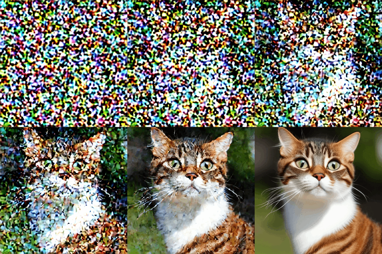
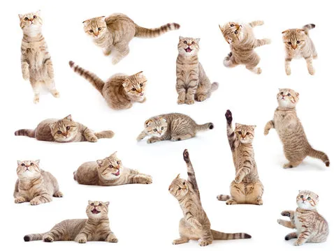
Image generation is all about synthesizing new images that match the statistical properties of a target dataset (for example, a collection of cat images). The main challenge is that we have plenty of sample cat images but we don’t have an explicit mathematical description of the underlying probability distribution of cat images. This means we must rely on learning methods that can generate new samples mimicking that unseen PDF.

Imagine having a huge collection of cat images but not knowing the precise recipe (the PDF) that tells you what makes a “cat image” a cat image. The goal is to learn how to generate new cat images that look as authentic as those in your dataset.

i.e. here are cat pictures, now generate me another picture from this distribution:

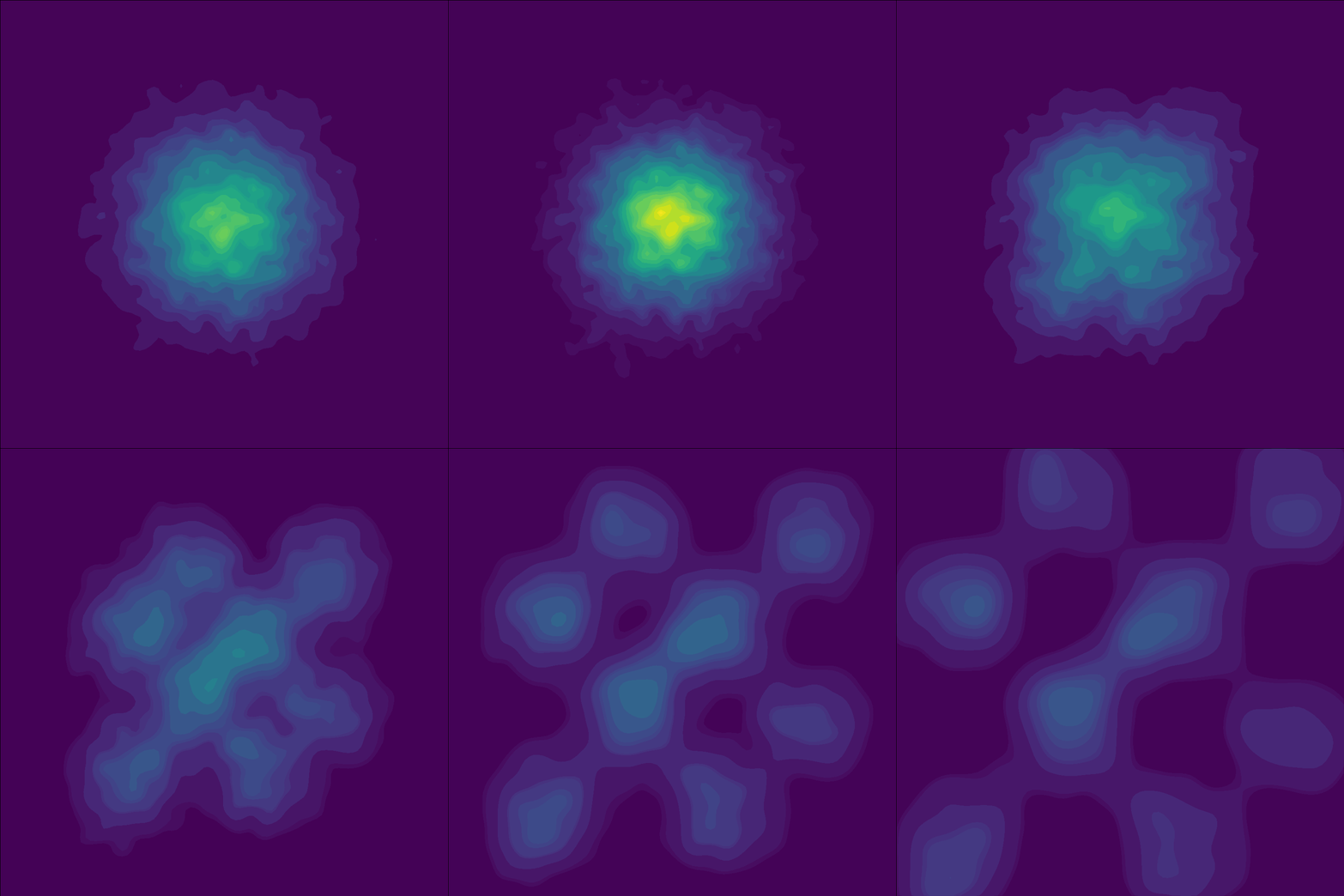
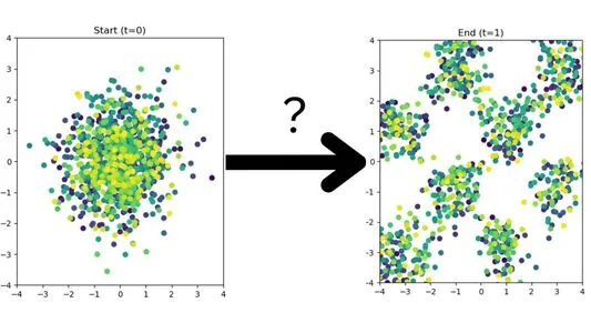
I simplify this problem to just having 2 dimensions (going from 2D gaussian to a checkerboard pattern) so we can visualize how this works.

Introduction to Flow Matching
#

Flow matching is a technique designed to learn a smooth transformation (flow) from a simple base distribution (like noise) to the target image distribution. Here’s the core idea:

Learning a Vector Field: We define a vector field, $\frac{dx}{dt} = f(x, t)$ that gradually transforms a random initial sample x(0) into a data sample x(1). This is akin to finding a path that “flows” the noise into a meaningful image.

With a simple update equation:

$x(t+\Delta t) = x(t) + \Delta t \cdot f(x(t), t)$

the model learns to iteratively adjust the sample along the trajectory determined by the flow field. This formulation is both intuitive and mathematically elegant, making it easier to train and understand compared to some more complex alternatives.

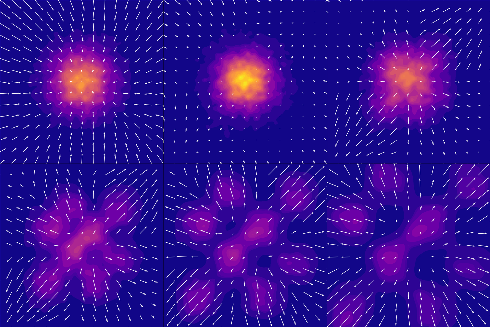
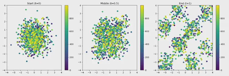
Here is the paths from a unit gaussian to a checkerboard my model learned: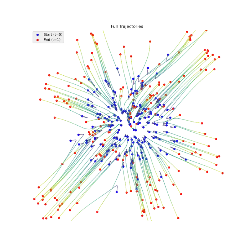

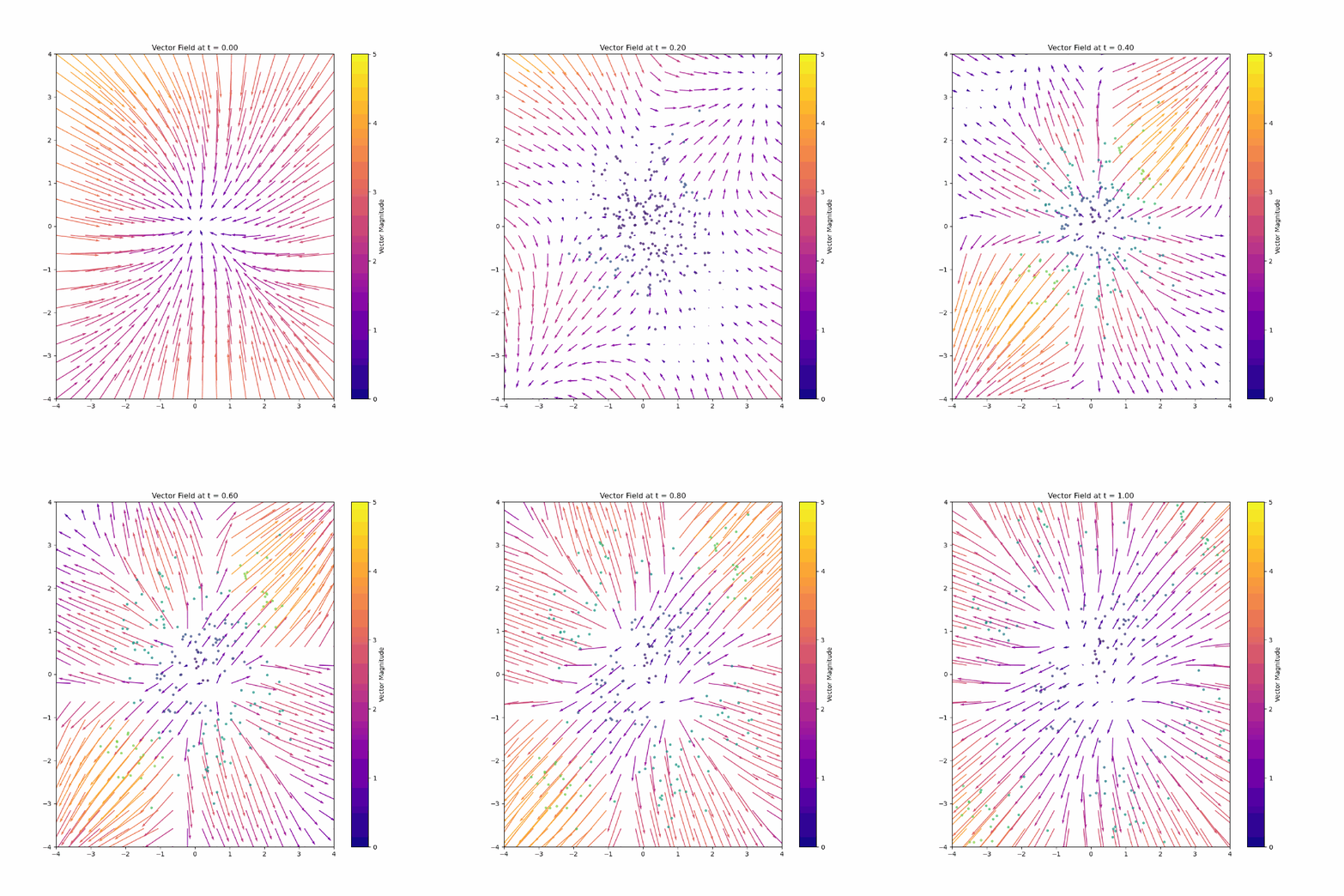
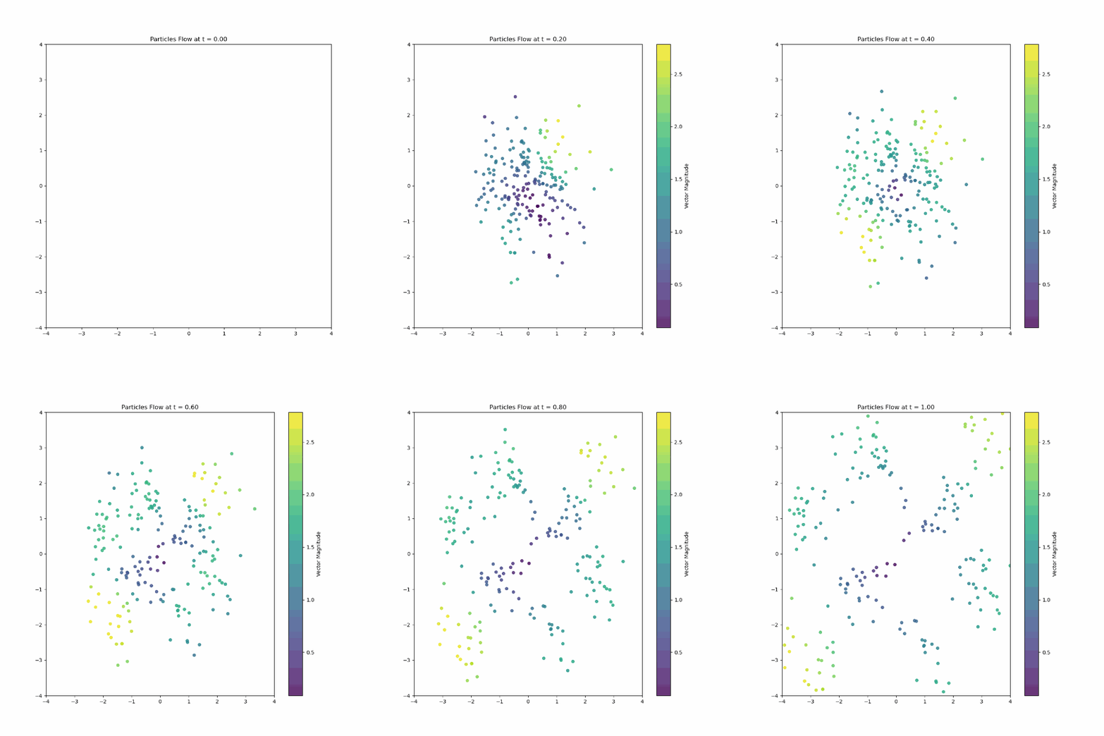
I love looking at the vectors on the top middle flick points to the left.

Flow Matching vs. Diffusion Models
#

While both flow matching and diffusion models are popular approaches for image generation, there are some key differences:

Diffusion Models:
#

These models work by gradually adding noise to an image and then learning how to reverse this process—a denoising step—to recover the original image. The process is inherently stochastic, involving randomness at each step. Diffusion models excel at handling uncertainty but can be computationally intensive due to the many steps required.

Flow Matching:
#

In contrast, flow matching directly learns a deterministic transformation (via the vector field) that transports samples from the noise distribution to the data distribution. This means:

Simplicity in Updates: The update rule is very straightforward, often resulting in simpler training dynamics.
Deterministic vs. Stochastic: Although noise can still be part of the process, the primary mechanism is a smooth, deterministic flow, which can be easier to analyze and debug. Overall, flow matching provides a clear picture of how image features evolve, which can be particularly insightful when comparing to the more diffuse nature of diffusion-based approaches.

Pseudocode for Training a Flow Matching Model
#

target_data = # put the samples you have from your target distribution here!

for i in tqdm(range(NUM_ITERATIONS)):
    # sample from source distribution (standard normal in this case)
    source_data = torch.randn(NUM_POINTS, 2)

    optimal_transport_line = target_data - source_data
    
    # sample random timestep t
    t = torch.rand(NUM_POINTS)
    
    # The input to the model at time t is just the linearly interpolated image
    input_data = source_data * t + target_data * (1 - t)
    
    # get velocity predictions from the flow matching model
    predictions = model.forward(input_data, t)
    
    # compare the velocity prediction to the straight line from source point to traget point
    loss = torch.nn.functional.mse_loss(predictions, optimal_transport_line)
    
    # gradient descent!
    optimizer.zero_grad()
    loss.backward()
    optimizer.step()

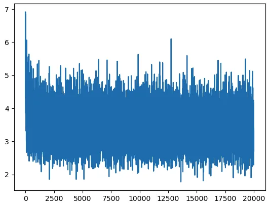
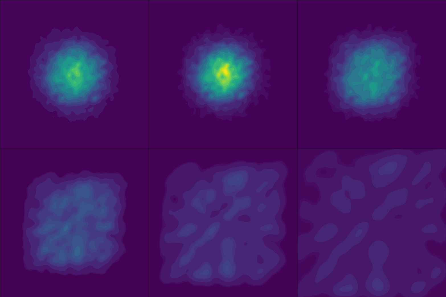
Keep in mind the loss will look like it isnt learning anything, but thats because of the random sampling of our source distribution (don’t worry about it. Just train for like 10,000 steps)

Pseudocode for Sampling a Flow Matching Model
#

We are just solving the differential equation with Eulers method. The idea is just to start at a point, use the model to get the direction we should go in, take a tiny step in that direction, then repeat.

coordinate = torch.randn(1) # get a point from our source distribution
dt = 1 / TimeSteps # Time step size dt

for i in range(TimeSteps):
    # Get vector field at current positions and time
    vector_field = model.forward(coordinate, i/TimeSteps)
    
    # Euler step integration: x_{t+dt} = x_t + v_t * dt
    coordinate = coordinate + vector_field * dt

Experimental Insights: High Frequency is Hard
#

During my experiments, I encountered an interesting detail that affected the quality of the generated images. I was using a checkerboard pattern as part of the visualization for the flow field, but the pattern’s granularity made a noticeable difference.

Fine vs. Coarse Checkerboard:
#

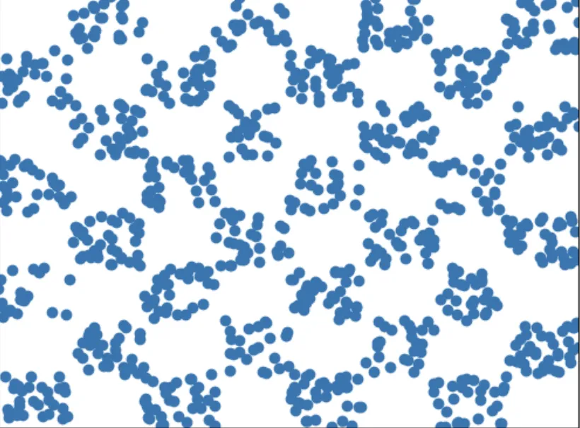
My initial experiments used a fine checkerboard pattern, meaning the squares were small. This level of fine detail made it hard for the model to guide the points precisely (so there were lots of points that ended up in spaces that were supposed to end up empty).

The Fix:
#

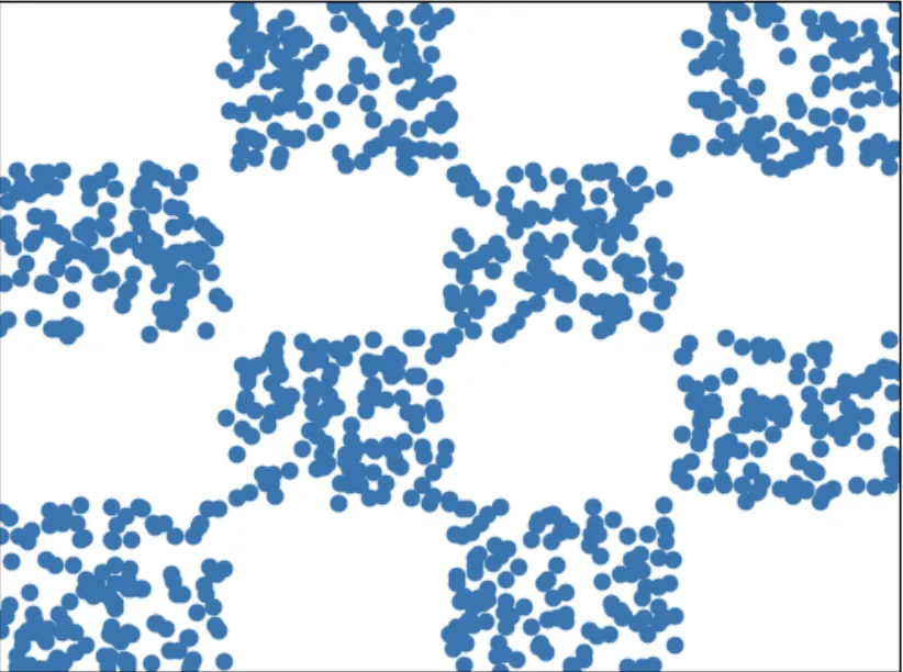
By uniformly increasing the size of each square (so that each square has roughly four times the area), the flow field could separate and transform the points much more effectively. (And I got a cleaner looking checkerboard pattern after flowing)

Sometimes, simple adjustments in the experimental setup can lead to significant improvements in results.

Final Thoughts
#

Flow matching offers an elegant and intuitive way to bridge the gap between a simple noise distribution and the complex world of image data. By directly learning a flow field, we can generate high-quality images with a relatively simple update mechanism, all while avoiding some of the complications inherent in diffusion models.

I hope this post clarifies the concepts behind flow matching and provides some insights into both its theoretical underpinnings and practical implementation. Feel free to check out the YouTube video that was very useful in shaping my understanding of flow matching.

Checkout my code here:

undefined

Jupyter Notebook

undefined