making a VICReg

Background Link to heading

In Lex Fridmans interview of Yann Lecun, Yann Lecun says there are a few things LLMs fundamentally can’t do in their current state that a human can.

Some of thee include:

• Planning
• Logical reasoning

He is an advocate of self-supervised learning, and in the interview, talks about JEPA and how self-supervised learning could allow models to construct a world model by just observing the world.

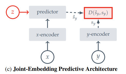
The joint embedding cuts out the irrelevant details of a feed (like cutting out specific leaf positions in a dashcam video) and keeps the important information (like which way the road is turning in a dashcam video).

Once this embedding is trained, a predictor can be trained on top of it to predict the next frames embedding from the previous frames embedding.

This is essentially trying to predict the next frame in a given video, but cutting out irrelevant details by doing the predictions in embedding space.

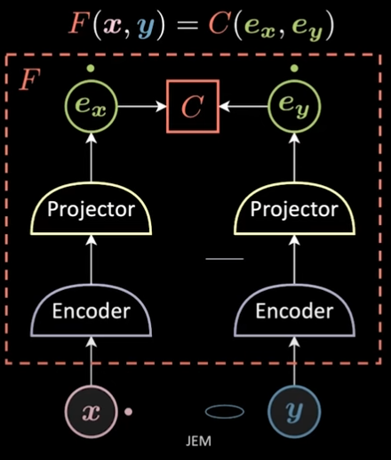
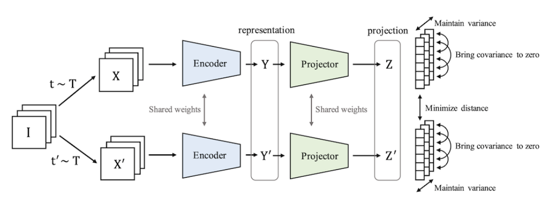
Yann Lecun mentions VICReg as an example embedding network, so I looked up the paper and tried it out on CIFAR-10.

results Link to heading

The final network has the following architecture:

class VICReg(nn.Module):
    def __init__(self, embedding_dimention, representation_dimention):
        super(VICReg, self).__init__()
        self.features = models.vgg16().features
        for param in self.features.parameters():
            param.requires_grad = False
        
        self.embedding = nn.Sequential(
            nn.Linear(512, 128),
            nn.ReLU(),
            nn.Dropout(),
            nn.Linear(128, 32),
            nn.ReLU(),
            torch.nn.BatchNorm1d(32),
            nn.Linear(32, embedding_dimention),
        )

        self.expand = nn.Sequential(
            nn.Linear(embedding_dimention, 80),
            torch.nn.BatchNorm1d(80),
            nn.ReLU(),
            nn.Linear(80, 80),
            torch.nn.BatchNorm1d(80),
            nn.ReLU(),
            nn.Linear(80, representation_dimention),
        )
    
        
    def forward(self, x):
        x = self.features(x)
        x = x.view(x.size(0), -1)
        x = self.embedding(x)
        x = self.expand(x)
        return x
    
    
model = VICReg(50, 100)

If you want to try this yourself, I used this tutorial.

The coolest thing about VICReg is the loss function. With just a MSE loss, all embdding would collapse to a single constant point (you get 0 loss if you map everything to a single point).

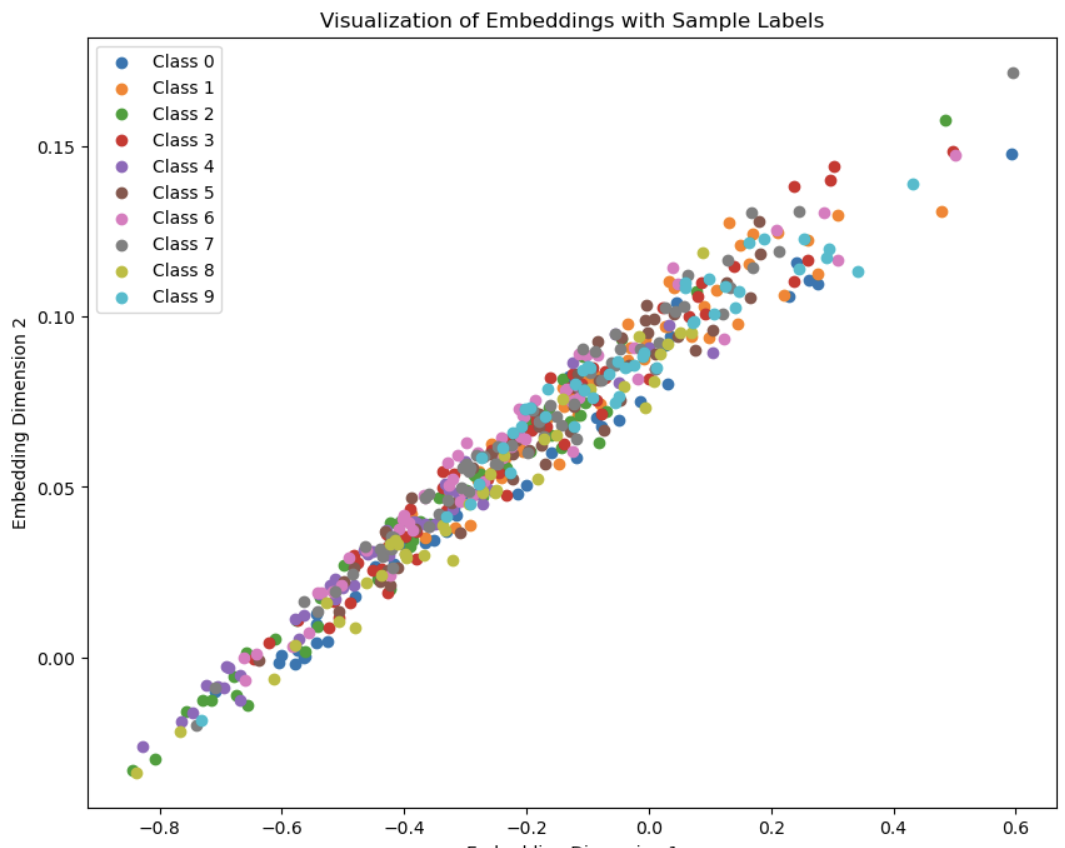
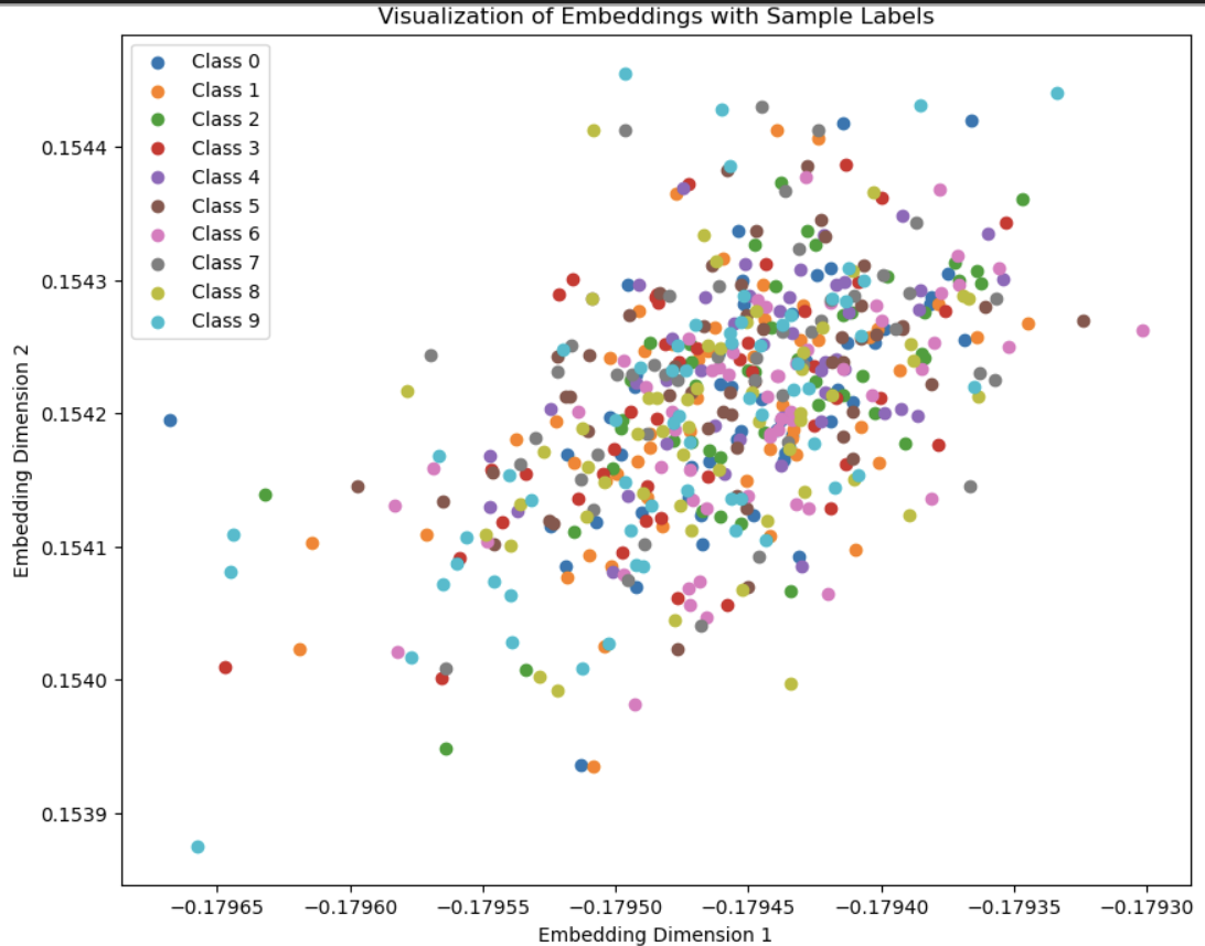
I omitted the pushing forces in my loss function and got a collapse of the 2-dimentional embedding space like this:

There are contrastive and non-contrastive methods for preventing collapse.

Instead of using a contrastive method (having positive and negative examples to pull and push examples from eachother), VICReg has a loss function with a regularization term so only positive examples are needed.

The loss function is made of 3 parts…

V loss Link to heading

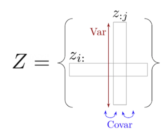
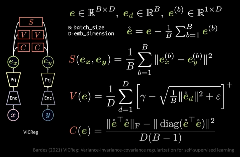
The V stands for variance. This looks at the variance of the embeddings over the batch. The more variance there is between embeddings in a batch, the lower the loss is. This pushes apart representations and prevents collapse.

The formula looks like this

For example, if batch size was 2 and we had the embeddings [1,2,3] and [1,2,3] for both samples, the variance loss would be high. If we had [0,0,0] and [1,1,1] for both samples, the variance loss would be low.

I loss Link to heading

The I stands for invariance. This is the normal MSE loss that pulls together similar samples.

C loss Link to heading

The C stands for covariance. This is not necessary but nice to have. This prevents dimentionality collapse. This means if we allow a dimention 3 embedding space, we encourage the model to use all 3 dimentions for embedding and discourage correlations between dimentions.

VICReg loss Link to heading

Combining it all together we get a pulling force from I loss, pushing force from V loss and C loss.

This is the code I used:

I_importance = 25
V_importance = 25
C_importance = 1

epsilon = 0.0001
relu = nn.ReLU()

def loss_var(image1):
    std_z_a = torch.sqrt(image1.var(dim=0) + epsilon)
    
    loss_v_a = torch.mean(relu(1 - std_z_a))
    return loss_v_a
mse = torch.nn.MSELoss()

def loss_cov(image1):
    N, D = image1.shape
    image1 = image1 - image1.mean(dim=0)
    cov_z_a = ((image1.T @ image1) / (N - 1)).square()  # DxD
    
    return (cov_z_a.sum() - cov_z_a.diagonal().sum()) / D
    

def VICReg_loss(image1, image2):
    S_error = mse(image1, image2)
    
    var_loss = loss_var(image1) + loss_var(image2)
    
    cov_loss = loss_cov(image1) + loss_cov(image2)
    
    return I_importance*S_error + C_importance*cov_loss + V_importance*var_loss 
    

The embedding space I got looks a bit funky but that is probably because I am visualizing a 50 dimentional embedding space in 2 dimentions with T-SNE.

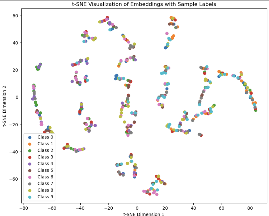
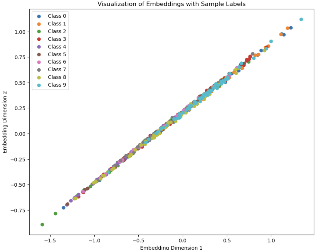
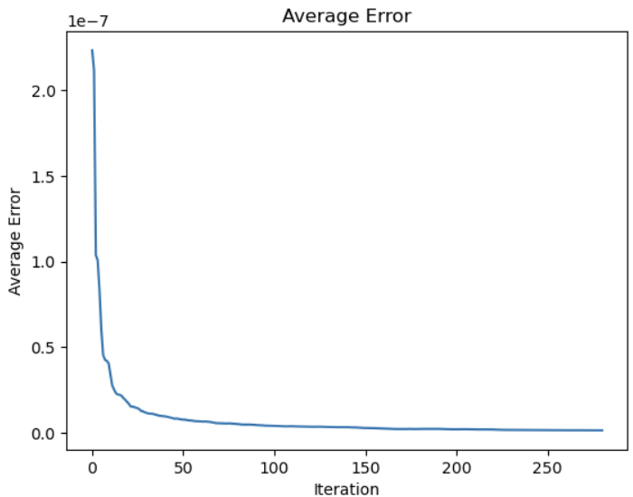
Loss averaged over 200 batches each:

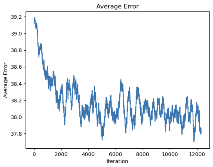
The diagonal pattern is probably because the covariance error is too small, which encourages points to be along the diagonal instead of using the whole space.

I tried making the weights 1,1,1 and increased the embedding dimention to 50 and the points spread out a bit.