Background#
Policy gradient methods directly optimize the expected return by taking gradients of the objective:
$$\nabla_\theta J(\theta) \approx \frac{1}{N} \sum_{i=1}^{N} \sum_{t=0}^{H-1} \nabla_\theta \log \pi_\theta(a_t^i | s_t^i) \hat{A}(s_t^i, a_t^i)$$where \(\hat{A}\) is the advantage estimate. The choice of advantage estimator determines the bias-variance tradeoff, which is the central theme of this assignment. We start with the full trajectory return (high variance), add reward-to-go (exploit causality), subtract a learned baseline (reduce variance further), and finally use GAE-λ (smoothly interpolate between TD and Monte Carlo).
1. Vanilla Policy Gradients on CartPole#
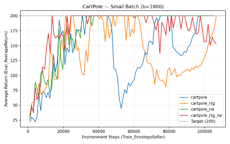
Eight experiments on CartPole-v0: all combinations of {small batch (1000), large batch (4000)} × {no tricks, reward-to-go, advantage normalization, both}.
# Small batch (b=1000): cartpole, cartpole_rtg, cartpole_na, cartpole_rtg_na
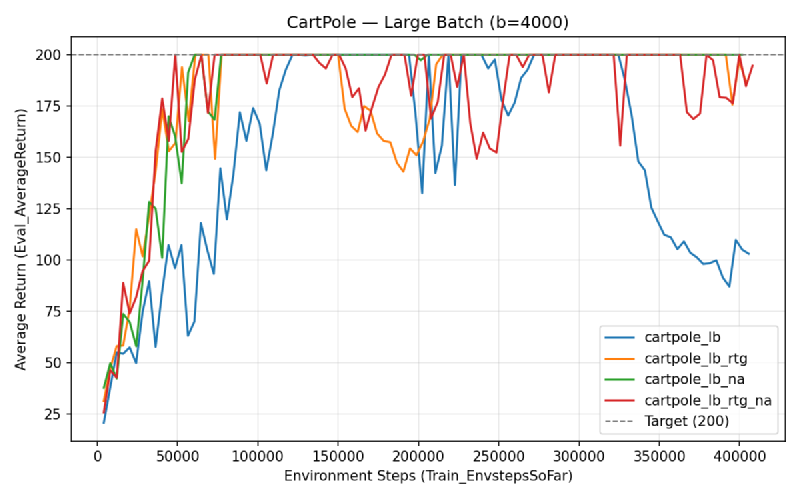
# Large batch (b=4000): cartpole_lb, cartpole_lb_rtg, cartpole_lb_na, cartpole_lb_rtg_na
./experiment1.sh
Small Batch (b=1000)#
Large Batch (b=4000)#
Questions#
Which value estimator has better performance without advantage normalization? Reward-to-go looks slightly better, though the difference is small in the small batch case.
Why is reward-to-go generally preferred? It has lower variance because it uses causality — rewards earned before a decision are irrelevant noise for that decision’s gradient.
Did advantage normalization help? Yes, quite a bit. The average reward reaches 200 quicker and stays more stable once there.
Did the batch size make an impact? Yes. Smaller batches converge faster in wall-clock iterations but are less stable after convergence. Larger batches trade speed for stability.
2. Neural Network Baselines on HalfCheetah#
A learned value function \(V_\phi^\pi(s_t)\) serves as a state-dependent baseline. The advantage becomes:
$$\hat{A}(s_t, a_t) = \sum_{t'=t}^{H-1} \gamma^{t'-t} r(s_{t'}, a_{t'}) - V_\phi^\pi(s_t)$$# No baseline vs baseline (bgs=5) vs baseline (bgs=2)
./experiment2.sh
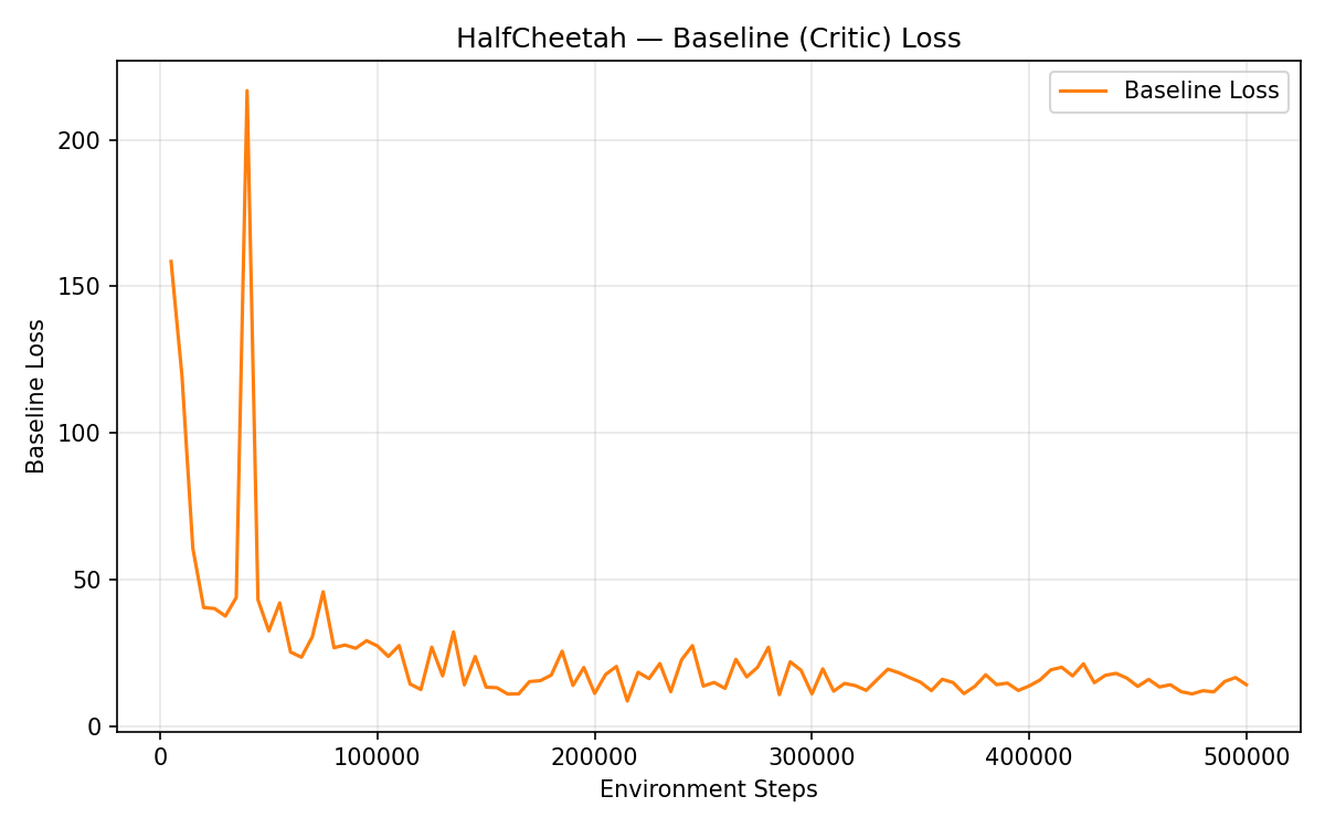
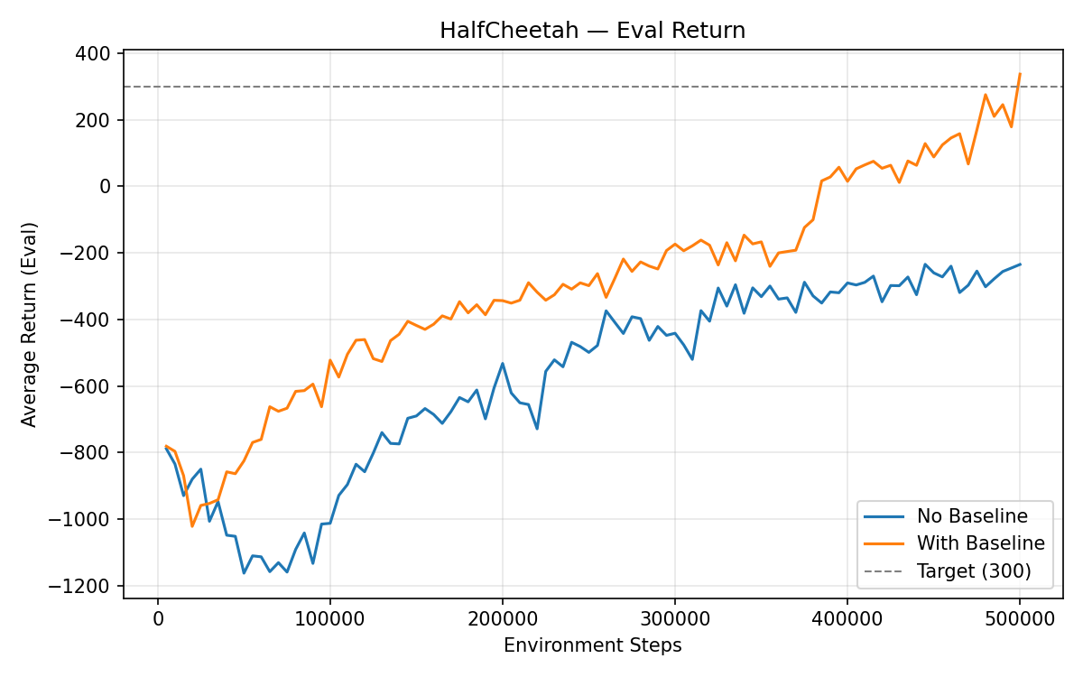
Effect of Reducing Baseline Gradient Steps (bgs=2 vs 5)#
I changed bgs from 5 to 2:
(a) The baseline learning curve becomes much more unstable — large spikes and a big uptrend toward the end, since 2 gradient steps aren’t enough to fit the value function well each iteration.
(b) The eval average return decreases significantly early on (~1000 steps) due to the high baseline loss. When the baseline loss spikes up later, the eval return drops again — a bad baseline actively hurts the policy.
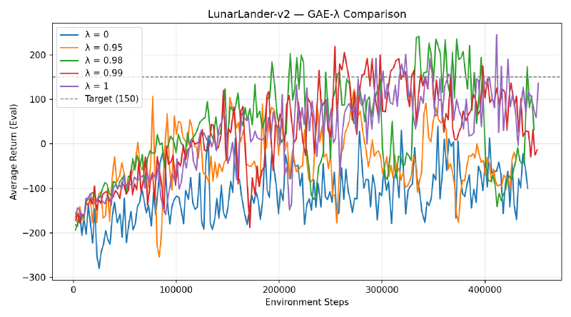
3. GAE-λ on LunarLander#
Generalized Advantage Estimation smoothly interpolates between TD(0) (λ=0, low variance / high bias) and Monte Carlo (λ=1, high variance / low bias):
$$\hat{A}^\text{GAE}(s_t, a_t) = \sum_{t'=t}^{H-1} (\gamma\lambda)^{t'-t} \delta_{t'}$$where \(\delta_t = r_t + \gamma V_\phi(s_{t+1}) - V_\phi(s_t)\).
# λ ∈ {0, 0.95, 0.98, 0.99, 1}
./experiment3.sh
Questions#
What does λ = 0 correspond to? Pure TD(1) — very low variance but high bias. The advantage estimate is just \(\delta_t\).
What about λ = 1? Full Monte Carlo returns — low bias but high variance.
In LunarLander, intermediate values of λ (0.95–0.99) perform well. λ = 0 underfits due to bias from value function errors, but λ = 1 doesn’t do too bad.
4. Hyperparameter Tuning on InvertedPendulum#
The default settings take ~328K env steps to reach max reward (1000). The goal: get there within 100K steps.
Approach#
I ran a random search (20 trials) sampling learning rates and batch size in log-space, then a second round of 20 trials centered on the best configuration from round 1.
Best Hyperparameters#
uv run src/scripts/run.py \
    --env_name InvertedPendulum-v4 \
    -n 100 \
    -b 2407 \
    -eb 1000 \
    --learning_rate 2.7e-02 \
    --baseline_learning_rate 3.3e-03 \
    --baseline_gradient_steps 23 \
    --discount 0.9996 \
    --n_layers 1 \
    --layer_size 64 \
    --use_reward_to_go \
    --exp_name pendulum_best
Random hyperparameter sweep code
"""Random hyperparameter search for InvertedPendulum-v4."""

import subprocess
import numpy as np

NUM_TRIALS = 20
GROUP = "pendulum_sweep_v2"
RNG = np.random.default_rng(123)


def log_uniform(low, high):
    return float(np.exp(RNG.uniform(np.log(low), np.log(high))))


def log_uniform_int(low, high):
    return int(round(log_uniform(low, high)))


def perturb_log(center, factor=3.0):
    """Sample log-uniformly within [center/factor, center*factor]."""
    return log_uniform(center / factor, center * factor)


def perturb_log_int(center, factor=3.0, low=1, high=None):
    val = int(round(perturb_log(center, factor)))
    val = max(val, low)
    if high is not None:
        val = min(val, high)
    return val


for i in range(NUM_TRIALS):
    batch_size = perturb_log_int(2653, factor=2.0, low=500)
    rtg = RNG.choice([True, False])
    blr = perturb_log(9.8e-3)
    bgs = perturb_log_int(16, factor=2.0, low=1, high=30)
    discount = 1.0 - perturb_log(1.0 - 0.9983, factor=5.0)  # perturb around 0.9983
    discount = min(discount, 0.9999)
    lr = perturb_log(2.8e-2)
    n_layers = int(RNG.integers(1, 3, endpoint=True))
    layer_size = int(RNG.choice([16, 32, 64]))

    tag = (
        f"b{batch_size}_lr{lr:.1e}_blr{blr:.1e}"
        f"_bgs{bgs}_d{discount:.4f}"
        f"_l{n_layers}_s{layer_size}"
        f"{'_rtg' if rtg else ''}"
    )
    exp_name = f"pendulum_{tag}"

    cmd = [
        "uv", "run", "src/scripts/run.py",
        "--env_name", "InvertedPendulum-v4",
        "-n", "100",
        "-b", str(batch_size),
        "-eb", "1000",
        "--learning_rate", f"{lr}",
        "--baseline_learning_rate", f"{blr}",
        "--baseline_gradient_steps", str(int(bgs)),
        "--discount", f"{discount}",
        "--n_layers", str(n_layers),
        "--layer_size", str(layer_size),
        "--exp_name", exp_name,
        "--group", GROUP,
    ]
    if rtg:
        cmd.append("--use_reward_to_go")

    print(f"\n{'='*60}")
    print(f"Trial {i+1}/{NUM_TRIALS}: {exp_name}")
    print(f"{'='*60}")
    subprocess.run(cmd, check=True)
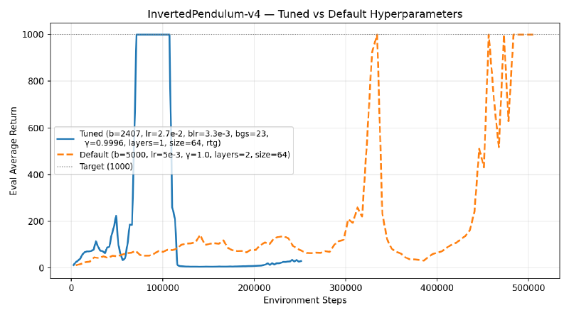
The tuned run reaches 1000 at ~71K env steps — a 4.5x speedup over defaults.
What Mattered#
- Learning rate was the most impactful. The default 5e-3 was too conservative; 2.7e-2 converged much faster. InvertedPendulum is simple enough that aggressive updates don’t destabilize training.
- Reward-to-go consistently helped — the best runs all had it enabled.
- Network architecture mattered less than expected. A single hidden layer of 64 units beat deeper/wider nets, suggesting a simple value function suffices for this task.
- Baseline gradient steps (23) — more fitting steps stabilized advantage estimation, paired with a lower baseline LR (3.3e-3 vs default 5e-3) to avoid overfitting.
- Batch size (~2400) balanced gradient quality with iteration speed.
- Discount factor (0.9996) — close to 1.0 but not exactly; unclear if this is meaningful or just noise from the random search.
Key Takeaways#
- Reward-to-go should always be used.
- Baselines reduce variance significantly but need enough gradient steps to be accurate; a bad baseline is worse than no baseline.
- GAE-λ provides a nice knob for bias-variance tradeoff.
- Hyperparameter tuning can yield big sample efficiency gains — 4.5x on InvertedPendulum from random search.
- Random search in log-space is a simple but effective tuning strategy for continuous hyperparameters.